Font and text formatting in Microsoft Excel allows you to modify the appearance of the text within cells. You can adjust various aspects of the font, such as its style, size, color, and effects. Text formatting is essential for making your data more visually appealing, organized and easier to read. In this article, we’ll explore the world of font and text formatting in Excel and discover how it can make your data more visually appealing and easier to understand.
1. Font Style:
The font style is like the personality of your text. Choosing the right font can significantly impact the readability and overall look of your worksheet.
Excel offers a variety of font styles to choose from, including options like Arial, Times New Roman, Calibri and more. You can select a font style that suits the overall look.
How to apply it:
- Select the cell or cells containing the text you want to format.
- Go to the “Home” tab in the Excel Ribbon.

- In the “Font” group, you’ll find various formatting options, including font style, font size, font color, bold, italics, underline, and more.
- Click on the font style drop-down list.

- Choose your desired font.

2. Font Size:
Font size determines how big or small the text appears within cells. Excel offers a range of font sizes, from very small to very large. You can increase or decrease the font size to improve readability or save space.
How to apply it:
- Select the cell and Go to the “Home” tab in the Excel Ribbon.
- In the “Font” group, click on the “Font size” drop-down list.

- Select the desired size.
3. Font Color:
Font color in Excel is a versatile formatting tool that allows you to change the color of text within cells. Change the color of the text to draw attention to specific information. Excel provides a wide range of color options for your text. You can choose from standard colors, theme colors or even define your custom color by selecting the “More Colors” option.
How to apply it:
- Select the cell or cells containing the text you want to change the color.
- Navigate to the “Home” tab in the Excel Ribbon.
- Under the “Font” group, click on the “Font color” option.

- Select the desired color from the available colors.
4. Bold, Italic and Underline:
Apply these formatting options to emphasize the text in Excel. Bold makes text thicker and more noticeable, italics slant the text and underline adds a line beneath the text.
How to apply it:
- Select the cell or cells containing the text you want to apply formatting.
- Navigate to the “Home” tab in the Excel Ribbon.

- Under the “Font” group, click on the “Bold” option or use the Keyboard shortcut Ctrl + B option to Bold the text in cells.
- Click on the “Italic” option or use the Keyboard shortcut Ctrl + I option to make the text slanted in cells.
- Click on the “Underline” option or use the Keyboard shortcut Ctrl + U option to add underline to your text in cells.
- Click on the “Double Underline” option to add a double underline to your text in cells.
5. Strikethrough:
Use strikethrough to draw a line through the text. This is often used to indicate that an item has been completed or is no longer relevant.
How to apply it:
- Select the cell or cells containing the text you want to apply formatting.
- Navigate to the “Home” tab in the Excel Ribbon.
- In the “Font” group, locate the font settings box launcher at the edge of the group.

- Click on it to open the format cells dialog box or use Ctrl + Shift +F to open the dialog box.
- Under the effects section, select the Strikethrough option and finally click OK.

- Alternatively, you can use the Keyboard shortcut Ctrl + 5 option to apply Strikethrough to your text in cells.

6. Superscript and Subscript:
You can format text as superscript (raised above the baseline) or subscript (lowered below the baseline). These are commonly used in mathematical expressions or chemical formulas like X2 and H2O.
How to apply it:
- Select the text or number in the cell.

- Navigate to the “Home” tab in the Excel Ribbon.
- In the “Font” group, locate the font settings box launcher at the edge of the group.
- Click on it to open the format cells dialog box or use Ctrl + Shift +F to open the dialog box.
- Under the effects section, select the Superscript and finally click OK.

- Now superscript will be added to the selected text.

- Now Select the text or number in the cell and Under the effects section, select the Subscript and finally click OK.

- Now subscript will be added to the selected text.

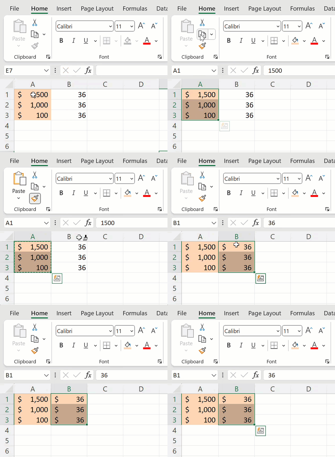
7. Format Painter:
This tool acts like a digital brush, allowing you to swiftly copy and apply formatting from one cell to another. It’s a real time-saver when you want consistent formatting throughout your worksheets and workbooks.
Here’s how to use it:
- Begin by selecting the cell containing the formatting you want to copy.

- Go to the “Home” tab in the Excel Ribbon and find the “Format Painter” button within the “Clipboard” group. It looks like a small paintbrush icon.

- Click the “Format Painter” button, Excel will temporarily change your cursor into a paintbrush icon.
- Next, click on the cell or range of cells where you want to apply the copied formatting.

- Instantly, the formatting from the source cell will be applied to the target cells.
Using font and text formatting effectively can help you create well-organized and visually appealing Excel documents, making it easier for readers to understand and interact with your data.
Discover more from Excellopedia
Subscribe to get the latest posts sent to your email.
