
If you’re opening Microsoft Excel for the first time, the screen can look overwhelming.
There are tabs, buttons, toolbars, menus, icons, rows, columns and dozens of options everywhere. Many beginners don’t know where to start, and that’s completely normal.
The good news is that you don’t need to learn every feature on your first day.
The first step is simply understanding the Excel Interface.
Once you know what each part of the Excel window is used for, learning formulas, functions, charts, PivotTables, and data analysis becomes much easier.
Think of the Excel Interface like the dashboard of a car.
Before driving, you first learn what the steering wheel, accelerator, brake, mirrors, and dashboard controls do.
Similarly, before becoming comfortable with Excel, you should understand where the important tools are located and what each one does.
In this complete beginner’s guide, we’ll explore every important part of the Microsoft Excel interface in a simple and practical way.
By the end of this guide, you’ll know exactly where to find Excel’s most important tools and how they help you work faster and more efficiently.
What is the Excel Interface?
The Excel Interface is the complete working screen that appears when you open Microsoft Excel.
It includes every tool, menu, button, tab, and workspace you’ll use while creating and managing spreadsheets.
Whether you’re entering data, writing formulas, creating charts, analyzing reports, or printing worksheets, everything begins with the Excel Interface.

In simple words, the Excel Interface is your workspace inside Microsoft Excel.
Every command you use is available somewhere within this interface.
Why is the Excel Interface Important?
Many beginners jump directly into learning formulas or functions without first understanding the Excel window.
As a result, they spend a lot of time searching for commands because they don’t know where the tools are located.
Once you’re familiar with the interface:
- You’ll find commands much faster.
- You’ll work more efficiently.
- Learning advanced Excel becomes easier.
- You’ll feel more confident using Excel.
That’s why understanding the Excel Interface is the first step in mastering Microsoft Excel.
What Will You Learn in This Guide?
In this article, you’ll learn:
- What each part of the Excel window is called.
- Where each feature is located.
- Why Microsoft provides each tool.
- When you should use each feature.
- Professional tips for working more efficiently.
We’ll explain every topic with simple language and practical examples so that even complete beginners can follow along with ease.
Let’s begin by exploring the first part of the Excel window: the Title Bar.
Title Bar in Microsoft Excel:
The Title Bar is the topmost section of the Microsoft Excel window. Although it may look simple, it provides important information about the workbook you’re currently working on and gives you quick access to several useful features.
Whenever you open Excel, the first thing you’ll notice at the top of the screen is the Title Bar.
It displays the name of the currently open workbook, along with several other options such as AutoSave, Search, and the Window Control Buttons.
Understanding the Title Bar helps you identify the workbook you’re working on and navigate Excel more efficiently.

Where is the Title Bar Located?
The Title Bar is located at the very top of the Excel window, above the Ribbon.
No matter which worksheet or Ribbon tab you’re using, the Title Bar always remains visible.
What Does the Title Bar Display?
The Title Bar displays several important pieces of information.
Workbook Name:
One of its primary functions is to display the name of the workbook.
When you create a new workbook, Excel automatically assigns a temporary name such as:
- Book1
- Book2
- Book3
These names remain until you save the workbook.
For example, if you save the workbook as:
Monthly Sales Report.xlsx
the Title Bar immediately updates and displays the new file name.
This makes it easy to identify which workbook you’re currently working on.
AutoSave:
If you’re using Microsoft 365 and your workbook is stored in OneDrive or SharePoint, you’ll see the AutoSave option on the left side of the Title Bar.
When AutoSave is turned on, Excel automatically saves your changes while you work.
This reduces the risk of losing your work due to a power failure or an unexpected system shutdown.
If you’re working with a file stored only on your computer, AutoSave may not be available.
Even if AutoSave is enabled, it’s still a good habit to press Ctrl + S occasionally, especially after making important changes.
Search Box:
Near the center of the Title Bar, you’ll find the Search box.
This is one of the fastest ways to locate Excel commands.
Instead of searching through different Ribbon tabs, simply type the name of the feature you’re looking for.
For example, you can search for:
- Freeze Panes
- Conditional Formatting
- PivotTable
- Data Validation
Excel immediately displays the matching commands.
This feature is especially helpful for beginners who haven’t yet memorized the location of different tools.

Window Control Buttons:
On the far-right side of the Title Bar, you’ll find the standard Windows control buttons.
These include:
- Minimize
- Maximize or Restore Down
- Close
Each button has a specific purpose.
- Minimize sends the Excel window to the Windows taskbar without closing it.
- Maximize expands the Excel window to fill the entire screen.
- If the window is already maximized, the button changes to Restore Down, allowing you to resize the window.
- The Close button closes the current Excel window.
Always make sure your workbook has been saved before clicking Close.
Why is the Title Bar Important?
Many beginners ignore the Title Bar, but it provides valuable information while working.
It helps you:
- Identify the active workbook.
- Quickly search for commands.
- Access AutoSave.
- Manage the Excel window.
If you’re working with multiple workbooks simultaneously, checking the Title Bar helps ensure you’re editing the correct file.
Real-World Example:
Imagine you’re preparing three different reports:
- Sales Report.xlsx
- Employee Salary.xlsx
- Inventory Report.xlsx
All three workbooks are open at the same time.
Before entering new data or making changes, simply look at the Title Bar.
The workbook name displayed there confirms which file you’re currently editing.
This simple habit can prevent costly mistakes.
Professional Tip:
- Professional Excel users always glance at the Title Bar before entering data or saving changes.
- This takes only a second but helps avoid editing the wrong workbook, especially when several Excel files are open at once.
Quick Access Toolbar in Microsoft Excel:
The Quick Access Toolbar (QAT) is one of the most useful productivity features in Microsoft Excel. Although it occupies only a small space on the screen, it can save you a significant amount of time while working.
The Quick Access Toolbar contains shortcuts to the commands you use most frequently. Instead of searching through different Ribbon tabs every time you need a command, you can access it instantly from the Quick Access Toolbar.
Whether you’re a beginner or an advanced Excel user, understanding and customizing the Quick Access Toolbar can make your daily work faster and more efficient.
Where is the Quick Access Toolbar Located?
By default, the Quick Access Toolbar is located in the top-left corner of the Excel window, just above the Ribbon.
No matter which Ribbon tab is currently open, the Quick Access Toolbar always remains visible.
This means your favorite commands are always just one click away.
Default Commands in the Quick Access Toolbar:
When you open Excel for the first time, the Quick Access Toolbar usually contains a few commonly used commands.
These include:
- Save
- Undo
- Redo
These commands are used so frequently that Microsoft places them in a permanent location for quick access.
Let’s understand each one.
Save:
The Save button allows you to save your workbook quickly.
Instead of going to File → Save, you can simply click the Save icon.
If the workbook hasn’t been saved before, Excel will ask you to choose a location and provide a file name.
After the first save, clicking the Save button updates the existing file with your latest changes.
Keyboard Shortcut: Ctrl + S
Undo:
Have you ever deleted data accidentally or made a formatting change you didn’t want?
There’s no need to panic.
Simply click the Undo button.
Excel immediately reverses your most recent action.
You can continue clicking Undo multiple times to reverse several recent actions.
Keyboard Shortcut: Ctrl + Z
Redo:
If you’ve undone an action by mistake, you can restore it using Redo.
Redo reverses the Undo operation and brings back the last action.
This is useful when you accidentally undo something you actually wanted to keep.
Keyboard Shortcut: Ctrl + Y
Why Use the Quick Access Toolbar?
Imagine you’re working on a large Excel workbook.
Throughout the day, you’ll save your work dozens of times.
You’ll also use Undo and Redo frequently while editing data.
Instead of navigating through menus repeatedly, the Quick Access Toolbar gives you instant access to these commands.
Even though each click saves only a second or two, those seconds add up over time, especially if you work in Excel every day.
Customizing the Quick Access Toolbar:
One of the biggest advantages of the Quick Access Toolbar is that it can be customized.
You can add your favorite commands so they’re always available, regardless of which Ribbon tab is open.
To customize it:
1. Click the small drop-down arrow at the end of the Quick Access Toolbar.

2. A list of commonly used commands will appear.
3. Simply select the commands you want to add.
4. The selected commands will immediately appear on the toolbar.
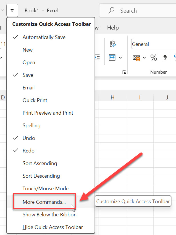
If the command you need isn’t listed, click More Commands.
From there, you can choose from hundreds of Excel commands and add them to your Quick Access Toolbar.

Useful Commands to Add:
As you become more comfortable with Excel, consider adding some frequently used commands, such as:
- New
- Open
- Quick Print
- Print Preview
- Sort Ascending
- Sort Descending
- Freeze Panes
- Format Painter
- Spelling
- Print Preview and Print
Having these commands available at all times can significantly improve your productivity.
Moving the Quick Access Toolbar:
By default, the Quick Access Toolbar appears above the Ribbon.
However, if you prefer, you can move it below the Ribbon.
To do this:
- Right-click anywhere on the Quick Access Toolbar.

- Select Show Below the Ribbon.

- If you later want to move it back, simply right-click again and choose Show Above the Ribbon.
This flexibility allows you to arrange the Excel interface according to your preference.
Real-World Example:
Imagine you’re preparing a monthly sales report.
While working, you repeatedly:
- Save your workbook.
- Undo accidental changes.
- Freeze the header row.
- Print the final report.
Instead of switching between multiple Ribbon tabs each time, you can add all these commands to the Quick Access Toolbar.
This keeps your most frequently used tools within easy reach and helps you complete your work more efficiently.
Professional Tip:
Professional Excel users rarely rely only on the default Quick Access Toolbar.
Instead, they customize it with the commands they use every day.
For example, an accountant may add Print Preview, Quick Print, and Spelling.
A data analyst may add Sort, Filter, and Freeze Panes.
By customizing the Quick Access Toolbar, you can create a workspace that matches your own workflow and saves valuable time.
Common Mistakes Beginners Make:
Here are a few common mistakes to avoid:
- Using only the default commands without exploring customization.
- Searching through Ribbon tabs for commands that could be added to the Quick Access Toolbar.
- Forgetting to save work regularly.
- Not using keyboard shortcuts like Ctrl + S, Ctrl + Z, and Ctrl + Y.
Avoiding these habits will help you work more efficiently.
The Ribbon in Microsoft Excel:
The Ribbon is one of the most important parts of the Microsoft Excel interface. Almost every command you use in Excel is available on the Ribbon.
Whether you’re formatting data, inserting charts, creating formulas, sorting information, or printing worksheets, you’ll usually begin by selecting the appropriate Ribbon tab.
If you’re new to Excel, the Ribbon may seem overwhelming because it contains hundreds of buttons and commands. However, Microsoft has carefully organized these commands into tabs and groups, making it easier to find the tools you need.
Once you understand how the Ribbon is organized, working in Excel becomes much faster and more efficient.
Where is the Ribbon Located?
The Ribbon is located just below the Title Bar and above the Formula Bar.
It extends across the top of the Excel window and remains available while you work.
Whenever you click a different Ribbon tab, the commands displayed on the Ribbon change automatically.
What is the Ribbon?
The Ribbon is a collection of tools and commands that help you perform different tasks in Excel.
Instead of displaying hundreds of commands in one place, Microsoft has divided them into logical categories called Tabs.
Each tab contains several Groups, and each group contains related commands.
This organized layout makes Excel much easier to learn and use.

Why Did Microsoft Introduce the Ribbon?
In older versions of Microsoft Excel, commands were stored inside multiple menus and toolbars.
Finding a specific command often required opening several menus, which made Excel difficult for beginners to learn.
To solve this problem, Microsoft introduced the Ribbon.
The Ribbon organizes commands based on the task you want to perform rather than hiding them inside menus.
This allows users to locate commands more quickly and work more efficiently.
Today, the Ribbon is used across most Microsoft Office applications, including Word, PowerPoint, and Outlook.
Understanding Ribbon Tabs:
The Ribbon is divided into several tabs.
Each tab is designed for a specific type of work.
The most commonly used Ribbon tabs include:
- Home
- Insert
- Page Layout
- Formulas
- Data
- Review
- View
Let’s briefly understand the purpose of each one.
This tab is particularly useful when sharing workbooks with others.
View Tab:
The View tab changes how your workbook is displayed on the screen.
It allows you to:
- Switch worksheet views
- Freeze Panes
- Split windows
- Zoom in or out
- Show or hide gridlines
- View multiple workbooks side by side
Remember, the View tab changes only the display of your worksheet. It does not change the actual data.
Ribbon Groups:
When you click a Ribbon tab, you’ll notice that the commands are divided into smaller sections.
These sections are called Groups.
For example, in the Home tab you’ll find groups such as:
- Clipboard
- Font
- Alignment
- Number
- Styles
- Cells
- Editing
Each group contains commands related to a specific task.
Dialog Box Launcher:
Some Ribbon groups contain a small diagonal arrow in the bottom-right corner.
This tiny button is called the Dialog Box Launcher.
Many beginners never notice it, but it opens additional settings that aren’t visible on the Ribbon.
For example, clicking the Dialog Box Launcher in the Font group opens the complete Font dialog box, where you’ll find advanced formatting options.
Whenever you see this small arrow, it’s worth clicking because it often provides additional features.
Contextual Tabs:
One interesting feature of the Ribbon is Contextual Tabs.
These tabs appear only when they’re needed.
For example:
- Select a picture, and the Picture Format tab appears.
- Select a chart, and Chart Design and Format tabs become available.
- Select a table, and the Table Design tab appears.
When you deselect the object, these tabs disappear automatically.
This keeps the Ribbon clean and displays only the tools relevant to your current task.
Can You Hide the Ribbon?
Yes.
If you need more space on your screen, you can temporarily hide the Ribbon.
There are several ways to do this:
- Press Ctrl + F1
- Double-click any Ribbon tab
- Use the Ribbon Display Options
To display the Ribbon again, simply repeat the same action.

This feature is especially useful when working on smaller laptop screens.
Professional Tips:
Here are a few tips that experienced Excel users follow:
- Learn the purpose of each Ribbon tab instead of memorizing individual buttons.
- Use keyboard shortcuts for frequently used commands.
- Explore the Dialog Box Launcher for advanced settings.
- Don’t ignore Contextual Tabs because they contain specialized tools.
- Collapse the Ribbon when you need more workspace.
Common Mistakes Beginners Make:
Many beginners make these mistakes:
- Trying to memorize every command in the Ribbon.
- Ignoring the Dialog Box Launcher.
- Forgetting that different tabs are designed for different tasks.
- Searching through every tab instead of using the Search box.
Avoiding these mistakes will make learning Excel much easier.
Home Tab in Microsoft Excel:
The Home tab is the first and most frequently used tab in Microsoft Excel. Whenever you create a new workbook or open an existing worksheet, Excel automatically displays the Home tab by default.
This is because the Home tab contains the commands you’ll use most often while working with data.
Whether you’re entering information, formatting cells, changing fonts, aligning text, applying colors, inserting rows, or finding data, you’ll find most of these tools in the Home tab.
If you’re learning Excel for the first time, this is the tab you’ll use more than any other.
Where is the Home Tab Located?
The Home tab is the first tab on the Ribbon, located just below the Title Bar.
Simply click Home, and Excel displays all the commands available in this tab.
The Home tab is divided into several groups, with each group designed for a specific type of task.
Let’s understand each group one by one.

Clipboard Group:
The first group in the Home tab is the Clipboard group.
As the name suggests, this group is mainly used for copying, cutting, pasting, and copying formatting.
The Clipboard group contains the following commands:
- Paste
- Cut
- Copy
- Format Painter
Paste:
The Paste command inserts content that has been copied or cut from another location.
For example, if you’ve copied a list of employee names, you can paste it into another worksheet or workbook.
Shortcut: Ctrl + V
Cut:
The Cut command removes the selected data from its current location and places it on the Clipboard.
You can then paste it somewhere else.
Unlike Copy, Cut moves the data instead of creating another copy.
Shortcut: Ctrl + X
Copy:
The Copy command creates a duplicate of the selected data without removing the original.
This is useful when the same information needs to appear in multiple places.
Shortcut: Ctrl + C
Format Painter:
The Format Painter copies only the formatting of a selected cell, such as:
- Font
- Font Size
- Font Color
- Fill Color
- Borders
- Number Format
- Alignment
It does not copy the actual data.
This is extremely useful when you want multiple cells to have the same appearance without formatting each one manually.
Font Group:
The Font group allows you to change the appearance of your data.
Here you can:
- Change the Font Style
- Increase or Decrease Font Size
- Make text Bold
- Apply Italic
- Add Underline
- Change Font Color
- Apply Fill Color
- Add Cell Borders
These options help you create attractive, professional-looking worksheets.
For example, you can use bold text for headings, different colors to highlight important values, and borders to organize your data clearly.
Alignment Group:
The Alignment group controls how the contents of a cell are positioned.
Using this group, you can:
- Align text to the Left, Center, or Right
- Align content to the Top, Middle, or Bottom
- Wrap long text within a cell
- Merge multiple cells
- Change Text Orientation
- Increase or Decrease Indentation
Good alignment improves readability and gives your worksheet a clean, organized appearance.
For example, instead of letting long text overflow into adjacent cells, you can use Wrap Text to display the entire content neatly within the same cell.
Number Group:
The Number group controls how numbers are displayed in Excel.
You can format data as:
- General
- Number
- Currency
- Accounting
- Percentage
- Date
- Time
- Fraction
- Scientific
- Text
You can also increase or decrease the number of decimal places displayed.
It’s important to remember that changing the number format usually changes only the appearance of the data, not the actual value stored in the cell.
For example, the value 0.5 can be displayed as 50% simply by applying the Percentage format.
The underlying value remains the same.
Styles Group:
The Styles group helps you apply professional formatting quickly.
It includes:
- Conditional Formatting
- Format as Table
- Cell Styles
Conditional Formatting:
Automatically highlights cells based on rules or conditions.
For example, you can highlight sales values greater than ₹50,000 or identify duplicate entries.
Format as Table:
Converts a normal data range into an Excel Table with built-in formatting, filters, and sorting features.
Cell Styles:
Provides ready-made formatting styles for headings, titles, totals, warnings, and other important information.
These tools save time and help maintain a consistent design throughout your workbook.
Cells Group:
The Cells group is used to modify the worksheet structure.
From here you can:
- Insert Cells
- Insert Rows
- Insert Columns
- Delete Cells
- Delete Rows
- Delete Columns
- Change Row Height
- Change Column Width
- Rename Worksheets
- Move or Copy Sheets
Whenever you need to make structural changes to your worksheet, you’ll use the Cells group.
Editing Group:
The final group is Editing.
This group contains several powerful tools that improve productivity.
Some of the most commonly used commands include:
- AutoSum
- Fill
- Clear
- Sort & Filter
- Find & Select
AutoSum:
Quickly calculates totals using the SUM function.
Fill:
Copies values, formulas, or patterns into adjacent cells.
Clear:
Removes data, formatting, comments, or hyperlinks from selected cells.
Sort & Filter:
Helps organize and display data efficiently.
Find & Select:
Allows you to search for specific values, formulas, formatting, or objects within your worksheet.
These commands become extremely useful when working with large datasets.
Real-World Example:
Imagine you’re preparing a monthly sales report.
Using the Home tab, you can:
- Copy sales data from another worksheet.
- Format the headings with bold text and colors.
- Align the titles in the center.
- Display sales figures as currency.
- Highlight the highest sales using Conditional Formatting.
- Convert the data into an Excel Table.
- Calculate the total sales using AutoSum.
As you can see, almost every basic task in Excel begins with the Home tab.
Professional Tips:
Here are a few best practices followed by experienced Excel users:
- Use Format Painter instead of repeating the same formatting.
- Apply Cell Styles for consistent worksheet design.
- Use Conditional Formatting to highlight important data automatically.
- Convert large datasets into Excel Tables for easier sorting and filtering.
- Learn keyboard shortcuts such as Ctrl + C, Ctrl + V, Ctrl + X, and Ctrl + Z to work faster.
Common Mistakes Beginners Make:
Many beginners:
- Format every cell manually instead of using Format Painter.
- Merge cells unnecessarily, which can create problems when sorting or filtering.
- Ignore Cell Styles and Conditional Formatting.
- Enter totals manually instead of using AutoSum.
Avoiding these mistakes will help you create cleaner and more professional worksheets.
Insert Tab in Microsoft Excel:
The Insert tab is one of the most powerful tabs in Microsoft Excel. As the name suggests, this tab allows you to insert different types of objects into your worksheet.
While the Home tab is mainly used for entering and formatting data, the Insert tab is used to make your worksheets more interactive, informative, and visually appealing.
Whether you want to create professional charts, insert pictures, build PivotTables, add icons, or create dashboards, you’ll find all these tools in the Insert tab.
If you’re preparing reports, presentations, or business dashboards, this tab will become one of your favorites.
Where is the Insert Tab Located?
The Insert tab is located on the Ribbon, immediately after the Home tab.
Simply click the Insert tab to display all the tools available for adding objects and visual elements to your worksheet.
The Insert tab is divided into several groups, each designed for a specific purpose.
Let’s explore them one by one.
Tables Group:
The first group is Tables.
This group allows you to organize your data into structured tables and create PivotTables for powerful data analysis.
The Tables group contains two important options:
- Table
- PivotTable
Table:
A normal range of data can be converted into an Excel Table with just one click.
Although your data may already look like a table, converting it into an official Excel Table provides several additional benefits.
For example:
- Automatic filtering
- Built-in sorting
- Alternate row colors
- Automatic table expansion
- Structured references in formulas
Excel Tables are much easier to manage than ordinary cell ranges.
They are especially useful when working with large datasets.
PivotTable:
The PivotTable is one of the most powerful features in Microsoft Excel.
Instead of manually calculating totals and creating reports, PivotTables allow you to summarize thousands of rows of data within seconds.
For example, suppose you have sales data for an entire year.
Using a PivotTable, you can quickly answer questions such as:
- Which product generated the highest sales?
- Which employee achieved the highest revenue?
- What were the monthly sales totals?
- Which region performed the best?
Without PivotTables, answering these questions could take a long time.
With PivotTables, it takes only a few clicks.
We’ll dedicate an entire module to PivotTables later in this course.
Illustrations Group:
The next group is Illustrations.
This group helps you insert graphical elements into your worksheet.
Available options may include:
- Pictures
- Online Pictures
- Shapes
- Icons
- SmartArt
- 3D Models
- Screenshot
These tools help make your worksheets more attractive and easier to understand.
Pictures:
You can insert images directly from your computer.
Pictures are commonly used for:
- Company logos
- Product images
- Employee photos
- Certificates
- Reports
Images make reports more professional and visually appealing.
Shapes:
Excel provides many ready-made shapes, including:
- Rectangles
- Circles
- Arrows
- Flowchart symbols
- Callouts
These are useful for creating diagrams, highlighting information, and designing dashboards.
Icons:
Icons are small professional graphics included in Microsoft Excel.
Instead of downloading icons from the internet, you can insert built-in icons directly into your worksheet.
Icons improve the appearance of reports and dashboards while maintaining a clean and professional design.
SmartArt:
SmartArt allows you to create professional diagrams without drawing everything manually.
Examples include:
- Organization Charts
- Process Diagrams
- Cycle Diagrams
- Hierarchies
- Timelines
SmartArt is widely used in business reports and presentations.
Add-ins Group:
Depending on your version of Excel, you may also see the Add-ins group.
Add-ins allow you to extend Excel’s functionality by installing additional tools and applications.
For example, some companies install custom add-ins for accounting, reporting, or data analysis.
Charts Group:
The Charts group is one of the most frequently used groups in the Insert tab.
Charts convert numbers into visual information.
Instead of looking at hundreds of rows of data, a chart helps you understand trends, comparisons, and patterns much more quickly.
Excel provides many chart types, including:
- Column Chart
- Bar Chart
- Line Chart
- Pie Chart
- Area Chart
- Scatter Chart
- Combo Chart
- Waterfall Chart
- Histogram
- Funnel Chart
Choosing the right chart makes your reports much easier to understand.
Sparklines Group:
Sparklines are small charts that fit inside a single cell.
Unlike regular charts, Sparklines don’t require additional space.
They provide a quick visual summary of trends.
Excel offers three types of Sparklines:
- Line
- Column
- Win/Loss
These are especially useful in dashboards where space is limited.
Filters Group:
The Filters group contains tools such as:
- Slicer
- Timeline
These tools work with Tables and PivotTables.
Instead of applying traditional filters, users can simply click buttons to filter their reports interactively.
This makes dashboards much more user-friendly.
Links Group:
The Links group allows you to create hyperlinks.
You can link to:
- Another worksheet
- Another workbook
- A folder
- A website
- An email address
Hyperlinks are particularly useful when creating navigation dashboards or interactive reports.
Text Group:
The Text group contains several useful options.
These include:
- Text Box
- Header & Footer
- WordArt
- Signature Line
- Object
For example, a Text Box allows you to place notes anywhere on the worksheet without affecting your data.
The Header & Footer option lets you display page numbers, dates, file names, or company names when printing worksheets.
Symbols Group:
The final group is Symbols.
This group allows you to insert:
Mathematical symbols
- Currency symbols
- Special characters
- Equations
These features are particularly useful for educational content, engineering documents, scientific calculations, and financial reports.
Real-World Example:
Imagine you’re preparing a Monthly Sales Dashboard.
Using the Insert tab, you can:
- Convert your sales data into an Excel Table.
- Create a PivotTable to summarize sales.
- Insert a Column Chart to visualize monthly performance.
- Add your company logo.
- Use Icons to highlight KPIs.
- Insert a Slicer for interactive filtering.
- Add SmartArt to explain the sales process.
Without the Insert tab, creating a professional dashboard would be much more difficult.
Professional Tips:
Here are a few tips followed by experienced Excel users:
- Convert large datasets into Excel Tables before creating charts.
- Use PivotTables for reporting instead of manual calculations.
- Choose the chart type that best represents your data.
- Use Icons and SmartArt sparingly to improve readability.
- Add Slicers to dashboards for easy filtering.
- Keep reports clean and avoid adding unnecessary graphics.
Common Mistakes Beginners Make:
Many beginners:
- Insert too many pictures and shapes, making worksheets cluttered.
- Choose the wrong chart type for their data.
- Ignore Excel Tables and continue using ordinary ranges.
- Try to summarize large datasets manually instead of using PivotTables.
- Overuse colors and decorative elements.
Keeping your worksheets simple and professional always gives better results.
Page Layout Tab in Microsoft Excel:
The Page Layout tab helps you control the appearance of your worksheet before printing. Whether you’re preparing a simple report or a professional business document, this tab provides all the tools needed to adjust the page layout and ensure your worksheet prints correctly.
Although many beginners don’t use this tab regularly, it becomes extremely important whenever you need to print worksheets or create well-formatted reports.
Instead of modifying your data, the Page Layout tab controls how your worksheet is arranged on the page.
If you’ve ever experienced problems like columns getting cut off, incorrect paper size, or improper page alignment while printing, the solution is usually found in the Page Layout tab.
Where is the Page Layout Tab Located?
The Page Layout tab is located on the Ribbon, between the Insert and Formulas tabs.
Clicking this tab displays several groups of commands related to worksheet layout and printing.
The major groups include:
- Themes
- Page Setup
- Scale to Fit
- Sheet Options
- Arrange
Let’s understand each group in detail.
Themes Group:
The first group is Themes.
A Theme is a predefined combination of colors, fonts, and visual effects that gives your workbook a consistent and professional appearance.
Instead of manually changing fonts and colors on every worksheet, you can apply a theme with a single click.
A theme typically includes:
- Font styles
- Theme colors
- Effects
If your workbook contains multiple worksheets, applying a theme ensures that every sheet follows the same design.
This is especially useful for business reports, company templates, and presentations.
Colors:
The Colors option allows you to change the color palette used throughout the workbook.
Once you select a different color theme, Excel automatically updates charts, tables, shapes, and other supported objects.
Fonts:
The Fonts option changes the default heading and body fonts used in your workbook.
Using consistent fonts gives your reports a clean and professional look.
Effects:
Effects control the appearance of objects such as shapes, SmartArt, and charts.
Although most beginners don’t use this feature frequently, it can enhance the visual style of dashboards and presentations.
Page Setup Group:
The Page Setup group is one of the most important groups in the Page Layout tab.
It contains several essential printing options, including:
- Margins
- Orientation
- Size
- Print Area
- Breaks
- Background
- Print Titles
These settings help prepare your worksheet for printing.
Let’s briefly understand each option.
Margins:
Margins determine the blank space between your worksheet content and the edges of the paper.
Choosing appropriate margins helps your worksheet look balanced and prevents content from being printed too close to the paper edges.
Orientation:
Orientation determines whether the worksheet is printed in:
- Portrait
- Landscape
Portrait is suitable for worksheets with fewer columns.
Landscape is useful for wider reports containing many columns.
Paper Size:
The Size option allows you to choose the paper size used for printing.
Common options include:
- A4
- Letter
- Legal
Always make sure the selected paper size matches the paper loaded in your printer.
Otherwise, the print output may not appear correctly.
Print Area:
Sometimes you don’t want to print the entire worksheet.
Instead, you may want to print only a specific section.
The Print Area option allows you to define exactly which cells should be printed.
This is particularly useful when working with large worksheets.
Check this beginner’s guide to know how to Print in Excel.
Breaks:
Excel automatically inserts page breaks whenever a worksheet spans multiple pages.
The Breaks option allows you to insert, remove, or reset page breaks manually.
This gives you greater control over where one printed page ends and the next begins.
Background:
The Background option lets you display an image behind the worksheet while working.
It’s important to note that worksheet backgrounds are for on-screen viewing only and are not printed with the worksheet.
Print Titles:
When printing large worksheets across multiple pages, the first row or first column may disappear on subsequent pages.
The Print Titles option solves this problem.
It allows you to repeat selected rows at the top of every printed page and selected columns on the left side of every printed page.
This makes multi-page reports much easier to read.
Scale to Fit Group:
The next group is Scale to Fit.
Sometimes your worksheet is slightly larger than the paper.
As a result, a few columns or rows may move onto another page.
The Scale to Fit options allow you to resize the worksheet so that it fits better when printed.
You can control:
- Width
- Height
- Scale
For example, you can instruct Excel to fit all columns onto one page while allowing the rows to continue onto additional pages.
This is one of the most useful features when preparing reports for printing.
Sheet Options Group:
The Sheet Options group controls whether certain worksheet elements are displayed on the screen or included in the printed output.
There are two main options:
- Gridlines
- Headings
For each option, you can choose whether it should be:
- Viewed on the screen
- Printed on paper
For example, if you want the worksheet gridlines to appear in the printed report, simply enable the Print checkbox under Gridlines.
Similarly, enabling Headings prints the row numbers and column letters.
Arrange Group:
The final group is Arrange.
This group becomes active only when you select an object such as:
- Picture
- Shape
- Icon
- Chart
- SmartArt
Arrange provides commands such as:
- Bring Forward
- Send Backward
- Selection Pane
- Align
- Group
- Rotate
These tools help you organize objects neatly within your worksheet.
They are especially useful when designing dashboards, forms, or visually rich reports.
Real-World Example:
Imagine you’re preparing a quarterly sales report for a management meeting.
Before printing, you can use the Page Layout tab to:
- Apply a professional theme.
- Change the page orientation to Landscape.
- Select A4 paper size.
- Define the Print Area.
- Repeat the header row on every page.
- Adjust scaling so all columns fit neatly.
- Print gridlines for better readability.
With just a few adjustments, your report becomes much more professional and easier to read.
Professional Tips:
Here are a few best practices followed by experienced Excel users:
- Always check the Page Layout settings before printing.
- Use Landscape orientation for wide reports.
- Match the selected paper size with the paper loaded in your printer.
- Repeat header rows using Print Titles for multi-page reports.
- Use Scale to Fit carefully to avoid making text too small.
- Preview your worksheet before printing to identify any layout issues.
Common Mistakes Beginners Make:
Many beginners:
- Print worksheets without checking the page layout.
- Select the wrong paper size.
- Ignore Print Titles for multi-page reports.
- Reduce scaling too much, making text difficult to read.
- Forget to define a Print Area when only part of the worksheet needs to be printed.
Avoiding these mistakes will help you produce professional-looking printouts.
Formulas Tab in Microsoft Excel:
The Formulas tab is one of the most powerful tabs in Microsoft Excel. It contains all the tools required to perform calculations, use built-in functions, manage named ranges, troubleshoot formulas, and control workbook calculations.
Excel is known for its ability to perform calculations quickly and accurately. Whether you’re calculating a student’s total marks, preparing a company’s payroll, analyzing sales data, or creating financial reports, the Formulas tab provides everything you need.
If you want to unlock the true power of Excel, understanding the Formulas tab is essential.
Where is the Formulas Tab Located?
The Formulas tab is located on the Ribbon between the Page Layout and Data tabs.
When you click the Formulas tab, you’ll see several groups containing tools for creating, managing, and auditing formulas.
The main groups include:
- Function Library
- Defined Names
- Formula Auditing
- Calculation
Let’s understand each group in detail.
Why is the Formulas Tab Important?
One of the biggest reasons Excel is widely used around the world is its ability to perform calculations automatically.
Instead of calculating values manually every time your data changes, Excel updates the results instantly using formulas and functions.
The Formulas tab gives you access to hundreds of built-in functions that can save time, reduce errors, and simplify complex calculations.
Function Library Group:
The first group is the Function Library.
This is where you’ll find hundreds of built-in Excel functions.
Instead of creating every calculation manually, you can simply choose the appropriate function from this library.
The Function Library organizes functions into different categories, making it easier to find the one you need.
Some of the most commonly used categories include:
- Financial
- Logical
- Text
- Date & Time
- Lookup & Reference
- Math & Trigonometry
- Statistical
- Engineering
- Information
Each category contains functions designed for specific tasks.
AutoSum:
One of the most frequently used tools in the Function Library is AutoSum.
AutoSum automatically inserts common functions such as:
For example, instead of typing the SUM formula manually, you can simply click AutoSum, and Excel automatically selects the most likely range of cells.
This is one of the quickest ways to calculate totals.
Insert Function:
Another useful option is Insert Function.
If you’re unsure which function to use, click the Insert Function button.
Excel opens a dialog box where you can:
- Search for functions
- Read function descriptions
- Select functions by category
This is particularly helpful for beginners who are still learning Excel functions.
Popular Function Categories:
Let’s briefly understand the major function categories available in Excel.
Financial Functions:
These functions are used for financial calculations such as:
- Loan payments
- Interest calculations
- Investments
- Depreciation
They are commonly used by accountants and finance professionals.
Logical Functions:
Logical functions help Excel make decisions based on conditions.
Examples include:
- IF
- AND
- OR
- NOT
For example, you can display “Pass” if marks are greater than 35 and “Fail” otherwise.
Text Functions:
Text functions help manipulate text data.
Examples include:
- LEFT
- RIGHT
- MID
- LEN
- UPPER
- LOWER
- PROPER
- CONCAT
These functions are useful when cleaning or formatting text.
Date & Time Functions:
These functions work with dates and times.
Examples include:
- TODAY
- NOW
- DATE
- YEAR
- MONTH
- DAY
They’re commonly used in attendance sheets, project tracking, and reports.
Lookup & Reference Functions:
These functions search for information within a worksheet.
Popular examples include:
- XLOOKUP
- VLOOKUP
- HLOOKUP
- INDEX
- MATCH
These are among the most powerful functions in Excel and are widely used in business environments.
Math & Trigonometry Functions:
These functions perform mathematical calculations.
Examples include:
These are used in almost every type of worksheet.
Statistical Functions:
Statistical functions help analyze numerical data.
Examples include:
These are useful for reports, research, and data analysis.
Defined Names Group:
The next group is Defined Names.
Normally, formulas refer to cells using addresses such as:
- A1
- B5
- D20
However, large worksheets can contain thousands of cell references, making formulas difficult to understand.
Excel allows you to replace cell references with meaningful names.
For example,
instead of:
=SUM(B2:B13)
you can create a named range called Sales and write:
=SUM(Sales)
This makes formulas much easier to read and maintain.
The Defined Names group includes options such as:
- Define Name
- Name Manager
- Create from Selection
- Use in Formula
Named ranges become especially useful in large workbooks shared among multiple users.
Formula Auditing Group:
The next group is Formula Auditing.
As worksheets become larger and formulas become more complex, finding mistakes can be challenging.
Formula Auditing provides tools that help you understand and troubleshoot formulas.
Important commands include:
- Trace Precedents
- Trace Dependents
- Remove Arrows
- Show Formulas
- Error Checking
- Evaluate Formula
- Watch Window
These tools make it much easier to identify calculation errors and understand how formulas are connected.
Professional Excel users rely on these tools when working with large financial models and business reports.
Calculation Group:
The final group is Calculation.
By default, Excel automatically recalculates formulas whenever the underlying data changes.
This setting is called Automatic Calculation.
However, very large workbooks containing thousands of formulas may recalculate slowly.
In such cases, Excel allows you to switch to Manual Calculation.
When Manual mode is enabled, formulas update only when you instruct Excel to recalculate.
For most users, Automatic calculation is the recommended setting.
Formula vs Function:
Many beginners believe that formulas and functions are the same.
They are closely related, but they are not identical.
A Formula is an expression created by the user.
Example:
=A1+B1
Here, you’re instructing Excel to add the values in two cells.
A Function, on the other hand, is a predefined formula already built into Excel.
Example:
=SUM(A1:A10)
Instead of writing a long calculation yourself, Excel performs it automatically using the SUM function.
In simple terms:
- Formula = Created by the user
- Function = Built into Excel
Understanding this difference is important because you’ll use both throughout your Excel journey.
Real-World Example:
Imagine you’re preparing a monthly sales report.
Using the Formulas tab, you can:
- Calculate total sales using SUM.
- Find the average monthly sales using AVERAGE.
- Count the number of transactions using COUNT.
- Retrieve customer details using XLOOKUP.
- Highlight performance using IF.
- Check formulas for errors using Formula Auditing.
Without these tools, preparing reports would take much longer and be more prone to errors.
Professional Tips:
Here are a few tips used by experienced Excel professionals:
- Start by learning basic functions such as SUM, AVERAGE, COUNT, MIN, and MAX.
- Use Named Ranges to make formulas easier to understand.
- Use Formula Auditing tools whenever formulas produce unexpected results.
- Keep Calculation Mode set to Automatic unless you’re working with very large workbooks.
- Learn keyboard shortcuts for working with formulas to improve productivity.
Common Mistakes Beginners Make:
Many beginners:
- Confuse formulas with functions.
- Type long calculations manually instead of using built-in functions.
- Ignore Formula Auditing tools.
- Use complex formulas without understanding cell references.
- Forget to check formulas after copying them.
Avoiding these mistakes will make your worksheets more accurate and easier to maintain.
Data Tab in Microsoft Excel:
The Data tab is one of the most powerful and practical tabs in Microsoft Excel. It contains tools that help you import, organize, clean, validate, sort, filter, and analyze data efficiently.
If you work with customer records, employee details, invoices, sales reports, inventory, financial statements, or any large dataset, you’ll spend a lot of time using the Data tab.
Whether you’re a beginner or an advanced Excel user, understanding the Data tab will help you work faster, reduce errors, and manage data more effectively.
Where is the Data Tab Located?
The Data tab is located on the Ribbon between the Formulas and Review tabs.
When you click the Data tab, you’ll find several groups of commands designed specifically for working with data.
The major groups include:
- Get & Transform Data
- Queries & Connections
- Sort & Filter
- Data Tools
- Forecast
- Outline
Let’s understand each group in detail.
Why is the Data Tab Important?
Data is the heart of every Excel workbook.
Before you can analyze data or create reports, your data must be accurate, organized, and easy to work with.
The Data tab provides tools that help you:
- Import data from different sources.
- Clean incorrect or duplicate data.
- Organize records.
- Validate user input.
- Filter information.
- Analyze trends.
Instead of performing these tasks manually, Excel provides powerful built-in tools that save both time and effort.
Get & Transform Data Group:
The first group is Get & Transform Data.
This feature allows Excel to import data from various external sources.
Instead of copying and pasting data every day, you can connect Excel directly to your data source.
You can import data from:
- Another Excel workbook
- CSV files
- Text files
- Databases
- Websites
- Online services
One of the biggest advantages is that imported data can be refreshed whenever the source data changes.
This feature is powered by Power Query, one of Excel’s most advanced data automation tools.
We’ll cover Power Query in detail later in this course.
Queries & Connections Group:
Whenever your workbook imports data from external sources, Excel stores information about those connections.
The Queries & Connections group helps you manage them.
Using this group, you can:
- View imported queries.
- Refresh existing data.
- Edit connections.
- Remove unused connections.
This is especially useful when creating dashboards or reports that are updated regularly.
Sort & Filter Group:
One of the most frequently used groups in Excel is Sort & Filter.
As your worksheet grows, finding specific information becomes difficult.
Sorting and filtering help you organize your data quickly.
Sort:
Sorting arranges your data in a specific order.
Common sorting options include:
- A to Z
- Z to A
- Smallest to Largest
- Largest to Smallest
- Oldest to Newest
- Newest to Oldest
For example,
you can sort employees alphabetically, arrange products by price, or organize invoices by date.
Sorting makes reports easier to read and analyze.
Filter:
Filtering allows you to display only the records that meet specific conditions.
For example,
suppose your worksheet contains sales data for all states.
Using Filters, you can display only:
- Andhra Pradesh
- Telangana
- Karnataka
without deleting or modifying the remaining data.
Filters are extremely useful when working with thousands of records.
Data Tools Group:
The Data Tools group contains some of Excel’s most useful productivity features.
These include:
- Text to Columns
- Flash Fill
- Remove Duplicates
- Data Validation
Let’s understand each one.
Text to Columns:
Sometimes all the information appears in a single column.
For example:
Ram, Hyderabad, India
Using Text to Columns, Excel can split this information into separate columns based on a delimiter such as a comma, space, or tab.
This feature is very useful when cleaning imported data.
Flash Fill:
Flash Fill is a useful Excel feature that recognizes patterns in your data and fills the remaining cells for you.
For example, if one column contains:
Krishna Kumar
You can enter:
Krishna
in the next column as the first example. Flash Fill can then recognize the pattern and extract the first names from the remaining rows.
It can save you a lot of manual work when cleaning or changing data.
Learn more: Flash Fill in Excel: How to Use It With Simple Examples
Remove Duplicates:
Large datasets often contain duplicate records.
The Remove Duplicates feature helps eliminate repeated entries with just a few clicks.
For example,
if the same customer appears multiple times, Excel can keep only one record and remove the duplicates.
This improves data accuracy and prevents reporting errors.
Data Validation:
Data Validation allows you to control what users can enter into a cell.
For example, you can:
- Create a drop-down list.
- Allow only whole numbers.
- Restrict dates.
- Prevent invalid entries.
This is one of the best ways to reduce data entry mistakes.
We’ll explore Data Validation in detail later in this course.
Forecast Group:
The Forecast group helps you predict future values based on historical data.
For example,
if you have monthly sales data for the past three years, Excel can estimate future sales trends.
Forecasting is useful for:
- Sales planning
- Budget preparation
- Inventory planning
- Business analysis
Although beginners may not use it immediately, it’s a valuable feature for business professionals.
Outline Group:
The final group is Outline.
Outline allows you to group rows or columns together.
Once grouped, you can expand or collapse them using a single click.
This is especially useful for:
- Financial reports
- Monthly summaries
- Budget worksheets
- Detailed project reports
Grouping makes large worksheets much easier to navigate.
Real-World Example:
Imagine you’re managing a customer database containing 20,000 records.
Using the Data tab, you can:
- Import customer data from a CSV file.
- Remove duplicate customers.
- Split full names into separate columns.
- Create drop-down lists for customer status.
- Sort customers alphabetically.
- Filter customers by city.
- Refresh imported data whenever new records become available.
Without the Data tab, these tasks would take hours to complete manually.
Professional Tips:
Experienced Excel users follow these best practices:
- Convert imported data into Excel Tables before analysis.
- Always remove duplicate records before creating reports.
- Use Data Validation to prevent incorrect data entry.
- Apply Filters instead of deleting unwanted rows.
- Learn Flash Fill because it can save hours of manual work.
- Refresh imported data instead of importing it repeatedly.
Common Mistakes Beginners Make:
Many beginners:
- Sort only one column instead of the entire dataset.
- Delete unwanted rows instead of using Filters.
- Ignore duplicate records.
- Enter inconsistent data because they don’t use Data Validation.
- Manually separate text instead of using Text to Columns.
Avoiding these mistakes will make your worksheets cleaner, more accurate, and much easier to manage.
Review Tab in Microsoft Excel:
The Review tab in Microsoft Excel provides tools that help you review, collaborate, proofread, and protect your workbook.
Although many beginners don’t use this tab regularly, it becomes extremely valuable when you’re working with colleagues, clients, or team members.
Whether you want to check spelling mistakes, add comments, leave notes, protect important worksheets, or improve workbook accessibility, you’ll find all these tools in the Review tab.
If your workbook will be shared with others, learning the Review tab is highly recommended.
Where is the Review Tab Located?
The Review tab is located on the Ribbon between the Data and View tabs.
Clicking this tab displays several groups of commands designed to help you review and protect your workbook.
The major groups include:
- Proofing
- Accessibility
- Comments
- Notes
- Protect
Let’s understand each group in detail.
Why is the Review Tab Important?
Creating a worksheet is only one part of the job.
Before sharing it with others, you should make sure that:
- The information is accurate.
- There are no spelling mistakes.
- Team members can leave feedback.
- Important formulas are protected.
- Sensitive worksheets cannot be modified accidentally.
The Review tab provides all these capabilities in one place.
Proofing Group:
The first group is Proofing.
The most commonly used feature here is Spelling.
Spelling:
Typing mistakes can make a report look unprofessional.
Instead of checking every word manually, Excel provides a built-in spelling checker.
When you click Spelling, Excel scans the worksheet and identifies words that may be incorrect.
It then suggests possible corrections, allowing you to review each one before making changes.
This feature is especially useful for:
- Employee names
- Product descriptions
- Reports
- Customer information
- Notes
Although Excel’s spelling checker isn’t as advanced as Microsoft Word’s, it is still very useful for finding common spelling mistakes.
Keyboard Shortcut: F7
Accessibility Group:
The next group is Accessibility.
Accessibility ensures that your workbook can be understood and used by everyone, including people who use assistive technologies.
The Check Accessibility feature scans your workbook and identifies potential issues.
Examples include:
- Missing Alt Text for pictures
- Poor color contrast
- Objects without descriptions
- Other accessibility concerns
If you’re preparing reports for a company, educational institution, or government organization, running an Accessibility Check is considered a good practice.
Comments Group:
The next group is Comments.
Comments allow multiple people to collaborate within the same workbook.
Instead of editing data directly, users can leave suggestions or ask questions.
For example, a manager might comment:
Please verify this sales figure.
Or a colleague may write:
Update this customer information after confirmation.
Comments help keep discussions organized and attached to the relevant cells.
This is much more efficient than sending separate emails for every change.
When Should You Use Comments?
Comments are useful when:
- Reviewing reports.
- Working in teams.
- Requesting clarification.
- Discussing changes.
- Tracking feedback.
Since Comments support conversations, team members can reply and continue discussions within the workbook.
Notes Group:
Excel also provides another feature called Notes.
Although Notes and Comments appear similar, they serve different purposes.
A Note is used to store simple information attached to a cell.
Unlike Comments, Notes are not designed for conversations.
For example, you might add a note such as:
- “Data collected on 15 July.”
- “Estimated value.”
- “Verified by Finance Team.”
Notes are useful for storing reference information that may be helpful later.
Comments vs Notes:
Many beginners confuse Comments and Notes.
Here’s the difference:
| Comments | Notes |
| Used for collaboration | Used for personal information |
| Supports conversations and replies | Displays a simple note |
| Best for teamwork | Best for reminders |
| Common in Microsoft 365 | Available in all versions |
A simple way to remember this is:
- Comments are for discussions.
- Notes are for information.
Protect Group:
The Protect group is one of the most important sections of the Review tab.
Sometimes you want users to view your workbook without changing important information.
The Protect group allows you to safeguard your worksheets.
Common options include:
- Protect Sheet
- Protect Workbook
- Allow Edit Ranges
Protect Sheet:
Protect Sheet prevents users from modifying selected parts of a worksheet.
For example, you can lock formulas while allowing users to enter data in input cells.
This is commonly used in:
- Invoice templates
- Attendance sheets
- Salary reports
- Budget worksheets
Protect Workbook:
Protect Workbook prevents structural changes.
For example, users cannot:
- Add worksheets
- Delete worksheets
- Rename worksheets
- Move worksheets
This helps preserve the workbook’s structure.
Allow Edit Ranges:
Sometimes different users require permission to edit different sections of a worksheet.
Allow Edit Ranges lets you specify which cells or ranges can be modified.
This feature is useful in shared business workbooks.
Real-World Example:
Imagine you’ve created a monthly sales report that will be reviewed by your manager and team.
Before sharing it, you can:
- Run a Spelling Check.
- Check Accessibility.
- Add Comments requesting sales verification.
- Add Notes explaining certain figures.
- Protect formulas from accidental editing.
- Prevent users from deleting worksheets.
These simple steps improve the quality, security, and professionalism of your workbook.
Professional Tips:
Experienced Excel users follow these best practices:
- Always run Spelling Check before sharing reports.
- Use Comments for team discussions.
- Use Notes for personal reminders or explanations.
- Protect worksheets that contain formulas.
- Keep only input cells unlocked if others need to enter data.
- Review Accessibility recommendations before distributing important workbooks.
Common Mistakes Beginners Make:
Many beginners:
- Ignore spelling mistakes.
- Confuse Comments with Notes.
- Share workbooks without protecting formulas.
- Allow everyone to edit important worksheets.
- Forget to review workbooks before sending them.
These small mistakes can lead to confusion, accidental edits, and inaccurate reports.
View Tab in Microsoft Excel:
The View tab in Microsoft Excel allows you to control how your workbook is displayed on the screen. Unlike many other tabs, the View tab does not change your data or formulas. Instead, it changes the way you see, navigate, and work with your workbook.
Whether you’re reviewing a large worksheet, comparing two workbooks, freezing headers, or adjusting the zoom level, the View tab provides several tools that make working in Excel more comfortable and efficient.
Although beginners often overlook this tab, experienced Excel users rely on it every day to improve productivity.
Where is the View Tab Located?
The View tab is located on the Ribbon, immediately after the Review tab.
When you click the View tab, Excel displays several groups of commands that help you customize the appearance of your workbook.
The main groups include:
- Workbook Views
- Show
- Zoom
- Window
- Macros
Let’s explore each group in detail.
Why is the View Tab Important?
When working with small worksheets, navigating Excel is usually simple.
However, as your worksheets become larger and more complex, you need better tools to:
- Navigate quickly.
- Compare worksheets.
- Keep important headings visible.
- Adjust the worksheet view.
- Work comfortably with large amounts of data.
The View tab provides all these features in one convenient location.
Workbook Views Group:
The first group is Workbook Views.
This group allows you to change how your worksheet is displayed.
The available options include:
- Normal
- Page Break Preview
- Page Layout
Each view serves a different purpose.
Normal View:
Normal View is the default view in Microsoft Excel.
This is the view you’ll use most of the time while:
- Entering data
- Editing worksheets
- Writing formulas
- Formatting cells
It provides a clean working environment without displaying page boundaries.
For everyday Excel work, Normal View is usually the best choice.
Page Break Preview:
The Page Break Preview displays how Excel will divide your worksheet into printed pages.
Blue lines indicate where page breaks occur.
If necessary, you can drag these page breaks to control exactly where one printed page ends and the next begins.
This feature is especially useful when preparing reports for printing.
Page Layout View:
The Page Layout view shows your worksheet almost exactly as it will appear when printed.
In this view, you can see:
- Margins
- Headers
- Footers
- Individual pages
This allows you to make adjustments before printing and helps ensure your report looks professional.
Show Group:
The next group is Show.
This group allows you to show or hide certain worksheet elements.
The available options include:
- Ruler
- Gridlines
- Formula Bar
- Headings
Ruler:
The Ruler is mainly available in Page Layout View.
It helps you measure and align objects more accurately on the page.
Although most Excel users don’t use the Ruler regularly, it can be helpful when designing printable reports.
Gridlines:
Gridlines are the light gray lines that separate cells in a worksheet.
If you uncheck the Gridlines option, the worksheet still contains cells, but the lines are hidden from view.
Many users hide gridlines while creating dashboards or presentation-style reports because it gives the worksheet a cleaner appearance.
Formula Bar:
The Formula Bar displays the contents of the active cell.
If you need additional workspace, you can temporarily hide the Formula Bar.
You can enable it again whenever needed.
Headings:
Headings refer to:
- Column letters (A, B, C…)
- Row numbers (1, 2, 3…)
If you hide the Headings, the worksheet still functions normally, but the row and column labels are no longer visible.
This option is useful when creating worksheets that you want to present or display on a large screen.
Zoom Group:
The next group is Zoom.
Sometimes the worksheet appears too small or too large on your screen.
The Zoom tools help you adjust the display size without changing your actual data.
The Zoom group includes:
- Zoom
- 100%
- Zoom to Selection
Zoom:
The Zoom option lets you choose a custom zoom percentage.
For example:
- 75%
- 100%
- 125%
- 150%
- 200%
Zooming in makes text easier to read, while zooming out allows you to see more of the worksheet.
100%:
Clicking 100% immediately returns the worksheet to its normal viewing size.
This is useful if you’ve zoomed in or out and want to return to the default view quickly.
Zoom to Selection:
Suppose you’ve selected a small table within a very large worksheet.
Instead of manually adjusting the zoom level, simply click Zoom to Selection.
Excel automatically enlarges the selected area so that it fills most of the screen.
This makes it much easier to focus on a specific part of your worksheet.
Window Group:
The Window group helps you manage multiple worksheets and workbooks.
It contains several useful commands, including:
- New Window
- Arrange All
- Freeze Panes
- Split
- Hide
- Unhide
- View Side by Side
- Switch Windows
Let’s understand the most commonly used options.
New Window:
The New Window command opens another window of the same workbook.
Both windows display the same workbook, allowing you to view different parts of it simultaneously.
This is very useful when working with large worksheets.
Arrange All:
If multiple workbooks are open, Arrange All organizes them neatly on your screen.
You can choose different layouts such as:
- Tiled
- Horizontal
- Vertical
- Cascade
This makes comparing multiple workbooks much easier.
Freeze Panes:
Freeze Panes is one of the most useful features in Excel.
It allows you to keep selected rows or columns visible while scrolling.
For example,
if your worksheet contains thousands of rows, you can freeze the header row.
As you scroll down, the headings remain visible, making your data much easier to read.
This feature is widely used in business reports and large data tables.
Split:
The Split option divides the worksheet into separate panes.
Each pane can be scrolled independently.
This allows you to compare different parts of the same worksheet without constantly scrolling back and forth.
Hide and Unhide:
The Hide command temporarily hides the current workbook window.
The workbook remains open but is no longer visible.
To display it again, use the Unhide command.
View Side by Side:
If you have two workbooks open, View Side by Side allows you to compare them simultaneously.
For example, you can compare:
This month’s sales report with last month’s report.
Two versions of the same workbook.
Budget versus actual expenses.
This feature saves a significant amount of time.
Switch Windows:
When multiple workbooks are open, Switch Windows lets you move quickly between them without minimizing or maximizing windows manually.
Macros Group:
The final group is Macros.
A Macro is a recorded sequence of actions that Excel can replay automatically.
Instead of performing the same task repeatedly, you can record it once and let Excel perform it whenever needed.
Macros are commonly used to automate repetitive tasks such as:
- Formatting reports
- Cleaning data
- Creating invoices
- Generating recurring reports
Although Macros are considered an advanced Excel feature, they can dramatically improve productivity.
We’ll explore Macros in a dedicated section later in this course.
Real-World Example:
Imagine you’re reviewing a sales report containing more than 15,000 rows.
Using the View tab, you can:
- Freeze the header row.
- Zoom in for better readability.
- Hide gridlines for a cleaner presentation.
- Compare two reports side by side.
- Switch between multiple workbooks.
- Use Page Layout View before printing.
These features make working with large worksheets much easier and more efficient.
Professional Tips:
Experienced Excel users follow these best practices:
- Use Freeze Panes whenever working with large tables.
- Switch to Page Layout View before printing reports.
- Hide gridlines when creating dashboards.
- Use View Side by Side to compare reports.
- Adjust the Zoom level according to your task.
- Use New Window to view different parts of the same workbook simultaneously.
Common Mistakes Beginners Make:
Many beginners:
- Scroll through large worksheets without using Freeze Panes.
- Ignore Page Layout View before printing.
- Work at uncomfortable zoom levels.
- Compare reports manually instead of using View Side by Side.
- Forget that the View tab changes only the display, not the actual worksheet.
Understanding these features can significantly improve your Excel experience.
Name Box in Microsoft Excel:
The Name Box is one of the most useful yet often overlooked features in Microsoft Excel. Many beginners use Excel for years without realizing how powerful this small box can be.
Although it occupies only a small area beside the Formula Bar, the Name Box can help you navigate large worksheets, select cell ranges instantly, and even create named ranges for easier formulas.
Once you start working with large workbooks, the Name Box becomes an excellent time-saving tool.
Where is the Name Box Located?
The Name Box is located at the left side of the Formula Bar, just above the worksheet area.
Whenever you select a cell, the Name Box displays the address of that active cell.
Although it looks like a simple text box, it performs several important functions that make working in Excel much faster.
What Does the Name Box Display?
The primary function of the Name Box is to display the address of the currently active cell.
For example:
If you click cell A1, the Name Box displays A1.
If you click C15, it displays C15.
If you click F250, it displays F250.
This allows you to identify the exact location of the active cell at any time.
Whenever you move to another cell, the Name Box updates automatically.
Jump to Any Cell Instantly:
One of the biggest advantages of the Name Box is that it allows you to move directly to any cell without scrolling.
Imagine your worksheet contains 10,000 rows.
Instead of scrolling all the way down, simply:
1. Click inside the Name Box.
2. Type the cell address.
3. Press Enter.
For example, type:
- A1000
- D2500
- AA500
Excel immediately jumps to the specified cell.
This feature can save a lot of time when working with large worksheets.
Select a Range of Cells:
The Name Box can also be used to select multiple cells instantly.
Instead of dragging your mouse across a large range, simply type the range address.
For example:
A1:D20
After pressing Enter, Excel selects every cell from A1 to D20.
Similarly, you can select:
- B5:B100
- C10:H50
- A1:Z500
This method is much faster and more accurate than manual selection, especially when working with large datasets.
Create Named Ranges:
One of the most powerful uses of the Name Box is creating Named Ranges.
Normally, formulas use cell references such as:
- B2:B13
- D5:D25
These references work correctly but may become difficult to understand in large workbooks.
Instead, you can assign a meaningful name to a range.
For example:
- Sales
- Employees
- Expenses
- Products
After selecting the range, type the desired name into the Name Box and press Enter.
The selected cells now have a meaningful name.
Later, instead of writing:
=SUM(B2:B13)
you can simply write:
=SUM(Sales)
This makes formulas much easier to read, understand, and maintain.
Rules for Naming a Range:
When creating Named Ranges, keep these simple rules in mind:
- The name must begin with a letter, an underscore (_), or a backslash ().
- Spaces are not allowed.
- Special characters such as , %, &, or cannot be used.
- The name should clearly describe the data.
For example:
✔ Sales2025
✔ Employee_List
✔ MonthlyExpenses
✖ Monthly Sales
✖ 2025Sales
Meaningful names make formulas much easier to understand.
Why Should You Use Named Ranges?
Named Ranges provide several advantages.
They:
- Make formulas easier to read.
- Reduce mistakes in formulas.
- Make large workbooks easier to maintain.
- Improve collaboration when sharing files with others.
Instead of trying to remember complex cell references, you can work with meaningful names.
Real-World Example:
Imagine you’re preparing a monthly sales report.
The sales values are stored in cells B2:B31.
Without Named Ranges, your formula would look like this:
=SUM(B2:B31)
After naming the range Sales, the same formula becomes:
=SUM(Sales)
Even someone seeing the workbook for the first time can immediately understand what the formula is calculating.
Professional Tips:
Experienced Excel users often use the Name Box to improve both speed and readability.
Some useful habits include:
- Use the Name Box to jump quickly to distant cells.
- Select large ranges without dragging the mouse.
- Create meaningful Named Ranges for frequently used data.
- Use simple and descriptive names instead of complicated cell references.
- Organize Named Ranges properly in large workbooks to make formulas easier to manage.
These small practices can save a significant amount of time when working with complex worksheets.
Common Mistakes Beginners Make:
Many beginners:
- Ignore the Name Box completely.
- Scroll manually instead of jumping directly to a cell.
- Create formulas using long cell references instead of Named Ranges.
- Use unclear or inconsistent names for ranges.
Learning to use the Name Box effectively can greatly improve your productivity in Excel.
Formula Bar in Microsoft Excel:
The Formula Bar is one of the most important components of Microsoft Excel. Every piece of data you enter into a worksheet, whether it’s text, numbers, dates, or formulas, can be viewed and edited through the Formula Bar.
Although beginners often type directly into cells, professional Excel users frequently use the Formula Bar because it provides more space for viewing and editing complex data.
If you’re planning to learn Excel formulas and functions, understanding the Formula Bar is essential.
Where is the Formula Bar Located?
The Formula Bar is located below the Ribbon and to the right of the Name Box.
Whenever you click on any cell in a worksheet, the Formula Bar displays the complete contents of that cell.
Unlike the worksheet, which may display only the final result, the Formula Bar always shows the actual content stored inside the selected cell.
What is the Formula Bar?
The Formula Bar is an input area where you can:
- View the contents of the active cell.
- Enter new data.
- Edit existing data.
- Create and modify formulas.
- Create and edit functions.
Think of the Formula Bar as a workspace where you can safely view and edit the contents of a cell without affecting the layout of your worksheet.
Viewing Cell Contents:
Whenever you select a cell, Excel displays its contents in the Formula Bar.
For example:
If cell A1 contains: Excellopedia
the Formula Bar displays: Excellopedia
If cell B2 contains: 25000
the Formula Bar displays: 25000
Similarly, if a cell contains a date, percentage, currency value, or text, the Formula Bar always displays the complete content.
This makes it easy to verify what has been entered into a cell.
Viewing Formulas:
One of the biggest advantages of the Formula Bar is that it displays the actual formula, not just the result.
For example, suppose cell D10 contains:
=SUM(D2:D9)
The worksheet might display: 185000
However, when you click the cell, the Formula Bar displays:
=SUM(D2:D9)
This allows you to understand exactly how Excel calculated the result.
Whenever you’re checking or troubleshooting formulas, the Formula Bar becomes extremely useful.
Editing Cell Contents:
The Formula Bar isn’t just for viewing information.
You can also edit the contents of any selected cell.
Simply:
1. Select the cell.
2. Click inside the Formula Bar.
3. Make the required changes.
4. Press Enter.
This method is especially useful when editing:
- Long text
- Complex formulas
- Nested functions
- Large calculations
Editing directly inside a small worksheet cell can sometimes be difficult, whereas the Formula Bar provides much more space.
Entering New Data:
You can also enter new information directly through the Formula Bar.
Simply:
- Select a cell.
- Click inside the Formula Bar.
- Type the required data.
- Press Enter.
The entered value will appear both in the selected cell and in the Formula Bar.
This method works for:
- Text
- Numbers
- Dates
- Formulas
- Functions
Expanding the Formula Bar:
Sometimes formulas become very long.
For example, advanced formulas containing multiple IF statements, XLOOKUP functions, or nested functions may not fit within a single line.
In such cases, Excel allows you to expand the Formula Bar.
Simply click the Expand Formula Bar button located at the right end of the Formula Bar.
The Formula Bar becomes larger, making long formulas much easier to read and edit.

Click the same button again to collapse it.
You can use the keyboard shortcut CTRL+SHIFT+U to expand/collapse the Formula Bar.
This feature is especially useful when working with advanced formulas.
Cancel and Enter Buttons:
Whenever you’re entering or editing data, Excel displays two buttons next to the Formula Bar.

These are:
- Cancel (X)
- Enter (✓)
Cancel:
The Cancel button discards any changes you’ve made before they’re saved.
You can also press the Esc key on your keyboard to cancel editing.
Enter:
The Enter button accepts the changes you’ve made and stores them in the active cell.
You can also press the Enter key on your keyboard.
Using keyboard shortcuts is generally faster and is the preferred method used by most experienced Excel users.
Formula Bar vs Cell Editing:
Many beginners wonder whether they should edit data directly inside the worksheet or use the Formula Bar.
The answer depends on the type of data.
For short values such as numbers or simple text, editing directly in the cell is perfectly fine.
However, for:
- Long paragraphs
- Large formulas
- Nested functions
- Complex calculations
the Formula Bar provides a much better editing experience.
It gives you more space and reduces the chances of making mistakes.
Real-World Example:
Imagine you’re preparing a salary calculation workbook.
One cell contains a long formula that calculates:
- Basic Salary
- HRA
- Allowances
- Deductions
- Tax
- Net Salary
The worksheet displays only the final salary amount.
But if you need to understand or modify the calculation, simply click the cell.
The Formula Bar displays the complete formula, allowing you to review and edit it without affecting the worksheet layout.
This makes maintaining large workbooks much easier.
Professional Tips:
Experienced Excel users follow these best practices:
- Always review formulas in the Formula Bar instead of relying only on the displayed result.
- Use the expanded Formula Bar for long and complex formulas.
- Edit formulas in the Formula Bar rather than inside the cell.
- Learn keyboard shortcuts such as Enter, Esc, and F2 to speed up editing.
- Check the Formula Bar whenever a calculated result looks unexpected.
These simple habits make formula editing easier and help reduce errors.
Common Mistakes Beginners Make:
Many beginners:
- Look only at the calculated result and ignore the actual formula.
- Try to edit long formulas inside the worksheet cell.
- Forget to press Enter after making changes.
- Accidentally overwrite formulas with values.
- Never expand the Formula Bar when working with complex formulas.
Understanding how to use the Formula Bar properly can prevent many common Excel mistakes.
Rows, Columns, Cells, Cell Addresses, and Ranges in Microsoft Excel:
Before you begin creating formulas, formatting worksheets, or analyzing data, it’s important to understand the basic building blocks of Microsoft Excel.
Every worksheet is made up of Rows, Columns, and Cells. Every piece of information you enter into Excel, whether it’s text, numbers, dates, or formulas, is stored inside a cell.
Understanding these concepts is essential because almost every Excel feature depends on them.
Think of a worksheet as a large grid made up of thousands of small boxes. Each box has its own unique location, allowing Excel to organize and manage data efficiently.
Let’s explore each of these concepts one by one.
Rows in Microsoft Excel:
A Row is a horizontal line of cells that runs from left to right across the worksheet.
Each row is identified by a unique number.
For example:
- Row 1
- Row 2
- Row 3
- Row 100
- Row 1000
The row numbers appear along the left side of the worksheet.
Whenever you click on a row number, Excel selects the entire row.
This is useful when you want to:
- Format an entire row.
- Insert a new row.
- Delete a row.
- Hide or unhide a row.
- Change the row height.
Rows are commonly used to store individual records.
For example:
| Row | Information |
| Row 2 | Customer 1 |
| Row 3 | Customer 2 |
| Row 4 | Customer 3 |
Each row usually represents one complete record.
Columns in Microsoft Excel:
A Column is a vertical line of cells that runs from top to bottom.
Unlike rows, columns are identified using letters.
For example:
- A
- B
- C
- D
- Z
After column Z, Excel continues with:
- AA
- AB
- AC
- AD
and so on.
The column letters appear at the top of the worksheet.
Clicking a column letter selects the entire column.
Columns are useful when you want to:
- Format an entire column.
- Change the column width.
- Insert or delete columns.
- Hide or unhide columns.
In most worksheets, each column represents one type of information.
For example:
| Column | Data |
| A | Employee ID |
| B | Employee Name |
| C | Department |
| D | Salary |
This organized structure makes data easier to understand and analyze.
Cells in Microsoft Excel:
A Cell is the intersection of a row and a column.
Whenever a row and a column meet, they form a cell.
For example:
- Column A + Row 1 = Cell A1
- Column C + Row 5 = Cell C5
- Column F + Row 12 = Cell F12
A cell is the smallest unit of a worksheet.
Every piece of information you enter into Excel is stored inside a cell.
Cells can contain:
- Text
- Numbers
- Dates
- Times
- Currency values
- Percentages
- Formulas
- Functions
Without cells, there would be no place to store or calculate data.
Active Cell:
Whenever you click on a cell, it becomes the Active Cell.
The active cell is highlighted with a thick border, making it easy to identify.
Only one cell can be active at a time.
Any information you type from the keyboard is entered into the active cell.
For example:
If cell B5 is active and you type 5000, Excel stores the value in B5.
Before entering data, always make sure you’ve selected the correct active cell.
This simple habit helps prevent mistakes.
Cell Address:
Every cell in Excel has a unique address.
A Cell Address is created by combining:
- The Column Letter
- The Row Number
For example:
| Column | Row | Cell Address |
| A | 1 | A1 |
| B | 5 | B5 |
| D | 12 | D12 |
| AA | 100 | AA100 |
The column letter always comes first, followed by the row number.
Think of a cell address like the address of a house.
Just as every house has a unique location, every cell in Excel has its own unique address.
These addresses are used in formulas, functions, charts, conditional formatting, and many other Excel features.
Cell References:
A Cell Reference is simply another name for a Cell Address.
Whenever you create a formula, Excel uses cell references to identify which cells should be included in the calculation.
For example:
=A1+B1
This formula tells Excel to add the values stored in cells A1 and B1.
Similarly,
=A2B2
multiplies the values in cells A2 and B2.
Understanding cell references is one of the most important skills in Excel because almost every formula depends on them.
Cell Range:
Sometimes you need to work with multiple cells instead of just one.
A group of cells is called a Range.
Ranges are identified using the first cell and the last cell, separated by a colon (:).
For example:
A1:A10
This includes every cell from A1 to A10.
Similarly,
A1:D10
includes every cell inside the rectangle formed by columns A to D and rows 1 to 10.
Ranges are used in:
- Formulas
- Functions
- Charts
- PivotTables
- Conditional Formatting
- Data Validation
Whenever you’re working with large amounts of data, you’ll use ranges frequently.
Selecting Multiple Cells:
Excel provides several ways to select multiple cells.
Using the Mouse:
- Click and drag across the required cells.
- This is the easiest method for selecting nearby cells.
Using the Shift Key:
- Click the first cell.
- Hold the Shift key.
- Click the last cell.
- Excel automatically selects every cell between them.
- This is useful for selecting large continuous ranges.
Using the Ctrl Key:
- Hold the Ctrl key while selecting different cells.
- This allows you to select multiple non-adjacent cells.
For example, you can select:
- A1
- C5
- E10
- H20
at the same time.
Selecting Entire Rows and Columns:
Sometimes you need to select an entire row or column.
To select a complete row:
- Click the Row Number.
- To select a complete column:
- Click the Column Letter.
This is commonly used when:
- Applying formatting.
- Changing row height.
- Adjusting column width.
- Inserting rows or columns.
- Deleting rows or columns.
Real-World Example:
Imagine you’re maintaining an employee database.
Each row represents one employee.
Each column stores a different type of information.
For example:
| Employee ID | Name | Department | Salary |
| 101 | Ravi | Sales | ₹ 35,000 |
| 102 | Priya | HR | ₹ 42,000 |
| 103 | Arun | Finance | ₹ 50,000 |
If you want to calculate the total salary, Excel uses the cell addresses in the Salary column to perform the calculation.
This simple row-and-column structure makes Excel an excellent tool for organizing and analyzing information.
Professional Tips:
Experienced Excel users recommend following these best practices:
- Always verify the active cell before entering data.
- Learn to identify cell addresses quickly.
- Use ranges instead of selecting cells one by one.
- Use the Shift and Ctrl keys to speed up selection.
- Organize your worksheet so that each row represents one record and each column represents one type of information.
These habits improve both accuracy and productivity.
Common Mistakes Beginners Make:
Many beginners:
- Confuse rows with columns.
- Enter data into the wrong active cell.
- Forget to use ranges in formulas.
- Select cells manually instead of using keyboard shortcuts.
- Leave blank rows or columns inside datasets, making analysis more difficult.
Avoiding these mistakes will help you build clean, well-organized worksheets.
Worksheet Area, Workbook, Worksheet, and Sheet Tabs in Microsoft Excel:
When you open Microsoft Excel, the largest portion of the screen is occupied by a grid of rows and columns. This is known as the Worksheet Area.
It is the primary workspace where you’ll spend most of your time entering data, creating formulas, formatting tables, analyzing information, and building reports.
Understanding the relationship between a Workbook, a Worksheet, the Worksheet Area, and Sheet Tabs is essential because every Excel project is built around these components.
Let’s explore each one in detail.
What is the Worksheet Area?
The Worksheet Area is the large grid of cells where all your work takes place.
Every worksheet consists of thousands of rows and columns, forming millions of individual cells where you can enter and manage data.
Whenever you:
- Type customer information
- Create formulas
- Build tables
- Insert charts
- Format reports
you are working inside the Worksheet Area.
Simply put,
The Worksheet Area is the main working space in Microsoft Excel where all data is entered, edited, and analyzed.
What Can You Do in the Worksheet Area?
Almost every task in Excel is performed inside the Worksheet Area.
For example, you can:
- Enter text and numbers.
- Perform calculations using formulas.
- Format cells.
- Create tables.
- Build charts.
- Apply conditional formatting.
- Sort and filter data.
- Create PivotTables.
Whether you’re a student, accountant, teacher, business owner, or data analyst, the Worksheet Area is where you’ll spend most of your time.
What is a Workbook?
A Workbook is the Excel file itself.
Whenever you create a new Excel file, you’re creating a workbook.
A workbook can contain one or multiple worksheets.
For example:
- Sales Report.xlsx
- Employee Database.xlsx
- Budget Planner.xlsx
Each of these files is a workbook.
Think of a workbook as a book.
Just as a book contains multiple pages, an Excel workbook can contain multiple worksheets.
What is a Worksheet?
A Worksheet is a single spreadsheet inside a workbook.
Each worksheet contains its own rows, columns, and cells.
You can use different worksheets to organize different types of information.
For example, a workbook named Annual Sales Report.xlsx might contain these worksheets:
- January
- February
- March
- April
- Summary
Each worksheet stores different data, but together they belong to the same workbook.
This keeps your information organized and easy to manage.
Workbook vs Worksheet:
Many beginners confuse these two terms.
Here’s an easy way to understand the difference.
| Workbook | Worksheet |
| An Excel file | A single sheet inside the file |
| Can contain multiple worksheets | Belongs to one workbook |
| Saved as .xlsx | Cannot exist independently |
| Similar to a notebook | Similar to a page in the notebook |
For example,
if your workbook is called:
School Management.xlsx
it might contain worksheets such as:
- Students
- Teachers
- Attendance
- Fees
- Results
Together, these worksheets make up one workbook.
What are Sheet Tabs?
At the bottom of the Excel window, you’ll notice small tabs.
These are called Sheet Tabs.
Each Sheet Tab represents one worksheet.
By clicking a Sheet Tab, you can instantly switch from one worksheet to another.
This makes it easy to organize related information within a single workbook.
Renaming a Worksheet:
When you create a new workbook, Excel automatically names the worksheets:
- Sheet1
- Sheet2
- Sheet3
These names don’t describe the contents of the worksheets.
It’s a good practice to rename them with meaningful names.
For example:
- Sales
- Customers
- Employees
- Expenses
- Dashboard
To rename a worksheet:
1. Double-click the Sheet Tab.
2. Type the new name.
3. Press Enter.
Meaningful sheet names make navigation much easier.
Adding a New Worksheet:
Whenever you need another worksheet, click the Plus (+) button next to the Sheet Tabs.
Excel immediately creates a new worksheet.
There is no practical limit for most users, so you can create as many worksheets as your workbook requires.
Moving a Worksheet:
Sometimes you may want to rearrange the order of your worksheets.
Simply click and drag the Sheet Tab to a new position.
For example, if you want the Dashboard worksheet to appear first, drag it to the beginning of the Sheet Tabs.
Organizing worksheets logically makes workbooks easier to use.
Copying a Worksheet:
Suppose you’ve already designed a worksheet with headings, formatting, and formulas.
Instead of creating another similar worksheet from scratch, you can simply make a copy.
To copy a worksheet:
1. Right-click the Sheet Tab.
2. Select Move or Copy.
3. Check Create a Copy.
4. Click OK.
Excel creates an identical worksheet, including all formatting, formulas, charts, and data.
This feature saves a significant amount of time.
Changing Sheet Tab Color:
Excel allows you to assign colors to Sheet Tabs.
To do this:
1. Right-click the Sheet Tab.
2. Choose Tab Color.
3. Select the desired color.

For example:
- Green for completed work.
- Yellow for worksheets in progress.
- Red for urgent reports.
- Blue for dashboards.
Colored Sheet Tabs make large workbooks much easier to navigate.
Hiding and Unhiding Worksheets:
Sometimes you don’t want to delete a worksheet, but you also don’t want it to be visible.
In that case, you can hide it.
To hide a worksheet:
1. Right-click the Sheet Tab.
2. Select Hide.
The worksheet disappears from view but remains part of the workbook.

Whenever you need it again:
1. Right-click any visible Sheet Tab.
2. Choose Unhide.
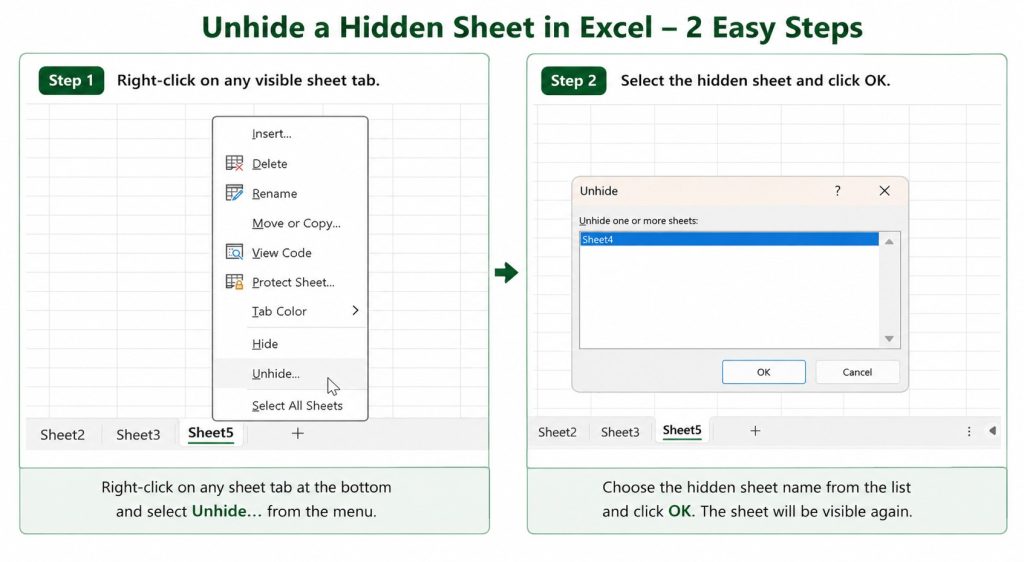
3. Select the worksheet.
4. Click OK.
This is useful for hiding calculations, supporting data, or confidential information without deleting it.
Deleting a Worksheet:
If a worksheet is no longer needed, you can delete it.
To delete a worksheet:
1. Right-click the Sheet Tab.
2. Select Delete.
Be careful.
Once a worksheet is deleted and the workbook is saved, recovering it can be difficult unless you have a backup.
Always verify that the worksheet is no longer required before deleting it.
Real-World Example:
Imagine you’re creating a workbook for managing a business.
Instead of placing everything on one worksheet, you organize it like this:
- Dashboard
- Customers
- Products
- Sales
- Purchases
- Expenses
- Employees
- Reports
Each worksheet stores a specific type of information, making the workbook well-organized and easy to navigate.
This is how most professional Excel workbooks are designed.
Professional Tips:
Experienced Excel users recommend these best practices:
- Give every worksheet a meaningful name.
- Arrange worksheets in a logical order.
- Use colors to identify important sheets.
- Keep dashboards at the beginning of the workbook.
- Hide supporting worksheets instead of deleting them.
- Copy existing worksheets to save time when creating similar reports.
Following these practices will make your workbooks more organized and easier to maintain.
Common Mistakes Beginners Make:
Many beginners:
- Leave worksheet names as Sheet1, Sheet2, and Sheet3.
- Store unrelated information on a single worksheet.
- Delete worksheets without creating a backup.
- Create multiple workbooks instead of organizing related data into one workbook.
- Forget to rename worksheets, making navigation confusing.
Avoiding these mistakes will help you build professional and well-structured Excel files.
Status Bar in Microsoft Excel:
The Status Bar is located at the bottom of the Microsoft Excel window and provides quick information about your worksheet and the data you’re working with.
Although many beginners rarely notice it, the Status Bar is one of Excel’s most useful productivity features. It displays the current status of your workbook, performs instant calculations, provides quick view options, and allows you to zoom in and out without opening additional menus.
Professional Excel users often rely on the Status Bar because it provides important information instantly, helping them save time while working.
Where is the Status Bar Located?
The Status Bar is positioned at the bottom of the Excel window, just below the worksheet area.
It stretches across the width of the application and remains visible while you work.
Depending on what you’re doing, the information displayed on the Status Bar changes automatically.

Why is the Status Bar Important?
The Status Bar provides quick information without requiring you to create formulas or navigate through multiple menus.
It helps you:
- Check the current worksheet status.
- View instant calculations.
- Switch worksheet views.
- Adjust the zoom level.
- Customize the displayed information.
Although it’s a small part of the Excel interface, it can significantly improve your productivity.
Worksheet Status:
The left side of the Status Bar displays the current status of your worksheet.
The most common status messages are:
- Ready
- Enter
- Edit
Each status tells you what Excel is currently doing.
Ready:
The Ready status indicates that Excel is waiting for your next action.
You can:
- Select a cell.
- Enter data.
- Click commands.
- Perform calculations.

This is the normal status you’ll see most of the time.
Enter:
When you begin typing into a cell, the Status Bar changes to Enter.
This means Excel is currently receiving new input.

After you finish typing and press Enter, the status usually returns to Ready.
Edit:
If you modify the contents of an existing cell, Excel displays Edit.
This indicates that you’re changing existing data instead of entering new information.

Understanding these status messages helps you know exactly what Excel is doing at any given moment.
Quick Calculations:
One of the most useful features of the Status Bar is its ability to perform instant calculations.
Simply select a range of cells containing numbers.
Without writing a single formula, Excel immediately displays useful information such as:
- Sum
- Average
- Count
- Numerical Count
This allows you to analyze data instantly.
Sum:
The Sum displays the total of all selected numerical values.
For example, if you select sales amounts from B2:B20, Excel immediately displays their total on the Status Bar.
This is much faster than creating a SUM formula when you only need a quick answer.
Average:
The Average displays the average value of the selected numbers.
Suppose you’ve selected employee salaries.
Excel instantly calculates and displays the average salary without requiring any formulas.
Count:
The Count option shows how many cells in the selected range contain data.
This is useful when you want to know how many entries exist in a dataset.
Numerical Count:
The Numerical Count counts only the cells containing numbers.
If your selection includes text as well as numbers, Numerical Count ignores the text and counts only the numeric values.
View Shortcuts:
Towards the right side of the Status Bar, you’ll find the View Shortcuts.
These allow you to quickly switch between different worksheet views without opening the View tab.
The available shortcuts include:
- Normal View
- Page Layout View
- Page Break Preview
These shortcuts save time and make it easier to preview your worksheet before printing.
Customizing the Status Bar:
One of the lesser-known features of Excel is that you can customize the Status Bar.
Simply:
1. Right-click anywhere on the Status Bar.
2. A customization menu appears.
3. Select or deselect the information you want Excel to display.

For example, you can choose to display:
- Average
- Count
- Numerical Count
- Sum
- Minimum
- Maximum
- Zoom Slider
- View Shortcuts
This allows you to personalize the Status Bar according to your workflow.
Real-World Example:
Imagine you’re reviewing a monthly sales report.
Instead of creating formulas to check the total sales or average sales value, simply select the relevant cells.
Immediately, the Status Bar displays:
- Total Sales
- Average Sales
- Number of Records
Within seconds, you have the information you need without modifying your worksheet.
This makes the Status Bar an excellent tool for quick analysis.
Professional Tips:
Experienced Excel users recommend these best practices:
- Check the Status Bar before creating temporary formulas.
- Use Quick Calculations for fast analysis.
- Customize the Status Bar to display only the information you use regularly.
- Use the View Shortcuts to switch between worksheet views quickly.
These habits can save time and improve your efficiency.
Common Mistakes Beginners Make:
Many beginners:
- Ignore the Status Bar completely.
- Create unnecessary SUM formulas for temporary calculations.
- Don’t realize the Status Bar can display averages and counts instantly.
- Never customize the Status Bar.
- Confuse Zoom with Print Scaling.
Learning how to use the Status Bar properly can make working in Excel much faster.
Scroll Bars and Zoom Slider in Microsoft Excel:
When working with small worksheets, it’s easy to see all your data on one screen. However, as your worksheets grow larger, navigating through hundreds or even thousands of rows and columns can become challenging.
This is where Scroll Bars and the Zoom Slider become extremely useful.
These simple navigation tools allow you to move quickly through large worksheets and adjust the worksheet display according to your needs.
Although they are basic features, you’ll use them almost every time you work in Microsoft Excel.
What are Scroll Bars?
Scroll Bars help you move around different parts of a worksheet without changing the actual data.
Excel provides two types of Scroll Bars:
- Vertical Scroll Bar
- Horizontal Scroll Bar
Together, they allow you to navigate through large worksheets quickly and comfortably.

Vertical Scroll Bar:
The Vertical Scroll Bar is located on the right side of the Excel window.
It allows you to move up and down through your worksheet.
For example, imagine you’re working with a worksheet containing 15,000 rows.
Instead of repeatedly pressing the Down Arrow key, simply drag the Vertical Scroll Bar downward to reach the required section instantly.
Likewise, dragging it upward takes you back to the beginning of the worksheet.
This makes navigation much faster when working with large amounts of data.
When Should You Use the Vertical Scroll Bar?
The Vertical Scroll Bar is useful when you need to:
- Review large reports.
- Navigate long customer lists.
- View employee records.
- Check inventory data.
- Analyze financial statements.
Instead of scrolling line by line, you can move to any section of the worksheet in just a few seconds.
Horizontal Scroll Bar:
The Horizontal Scroll Bar is located at the bottom of the worksheet, just above the Status Bar.
It allows you to move left and right across the worksheet.
This is especially useful when your worksheet contains many columns.
For example, if your report extends from Column A to Column AZ, you can drag the Horizontal Scroll Bar to quickly move across the worksheet.
Without it, navigating wide worksheets would be much slower.
When Should You Use the Horizontal Scroll Bar?
The Horizontal Scroll Bar is particularly useful for:
- Financial reports
- Sales dashboards
- Inventory sheets
- Employee databases
- Project tracking worksheets
Whenever your data extends beyond the visible screen width, the Horizontal Scroll Bar makes navigation much easier.
Scrolling with the Mouse Wheel:
If you’re using a mouse, you don’t always need to use the Scroll Bars.
Simply rotate the mouse wheel to move vertically through the worksheet.
Rotate the wheel down to scroll down.
Rotate the wheel up to scroll up.
This is one of the most common navigation methods used by Excel users.

Horizontal Scrolling Using the Mouse:
Many users don’t know that horizontal scrolling is also possible with certain mouse models.
On many systems, holding the Ctrl & Shift keys while rotating the mouse wheel scrolls the worksheet horizontally.
If your mouse supports horizontal scrolling, this can be a very convenient shortcut for working with wide worksheets.
What is the Zoom Slider?
The Zoom Slider is located at the bottom-right corner of the Excel window.
It allows you to change the size of the worksheet on your screen.
This feature improves readability without changing your actual data.

The Zoom Slider is particularly useful when:
- The text appears too small.
- You want to focus on a specific section.
- You need to see more of the worksheet at once.
Zooming In:
Move the Zoom Slider to the right to zoom in.
As the zoom percentage increases, everything on the worksheet appears larger.
Zooming in is useful when:
- Reading small text.
- Editing formulas.
- Reviewing detailed reports.
- Working on dashboards.
- Presenting Excel data during meetings.
Larger text makes editing easier and reduces eye strain.
Zooming Out:
Move the Zoom Slider to the left to zoom out.
This reduces the display size and allows you to see more rows and columns on the screen.
Zooming out is helpful when:
- Reviewing an entire worksheet.
- Checking page layouts.
- Viewing dashboards.
- Comparing different sections of a worksheet.
It gives you a broader view of your data without changing the worksheet itself.
Zoom Percentage:
Next to the Zoom Slider, Excel displays the current zoom percentage.
Common zoom levels include:
- 75%
- 100%
- 125%
- 150%
- 200%
Clicking the zoom percentage opens the Zoom dialog box, where you can choose a specific zoom level.
For everyday work, 100% is comfortable for most users.
However, you can adjust the zoom based on your screen size and personal preference.
Does Zoom Affect Printing?
This is one of the most common questions asked by beginners.
The answer is No.
Changing the zoom level affects only the display on your screen.
It does not change:
- Font size
- Cell size
- Worksheet size
- Print layout
- Printed output
If you need to adjust how your worksheet prints on paper, use Scaling or Page Setup, not the Zoom Slider.
Understanding this difference helps avoid confusion while preparing worksheets for printing.
Scroll Bars vs Zoom Slider:
Although both features help you work with large worksheets, they serve different purposes.
| Scroll Bars | Zoom Slider |
| Used for navigation | Used to change the viewing size |
| Moves through the worksheet | Enlarges or reduces the worksheet display |
| Does not change the zoom level | Does not move to another location |
| Helps access different rows and columns | Helps improve readability |
Knowing the difference between these two tools makes working in Excel much more efficient.
Real-World Example:
Imagine you’re reviewing a sales report with 5,000 rows and 40 columns.
You can:
- Use the Vertical Scroll Bar to move through thousands of sales records.
- Use the Horizontal Scroll Bar to view additional columns.
- Zoom in while editing formulas.
- Zoom out to review the overall worksheet layout.
Using these tools together makes navigation faster and much more comfortable.
Professional Tips:
Experienced Excel users recommend these best practices:
- Zoom in when editing formulas or reviewing small text.
- Zoom out when checking the overall layout of a worksheet.
- Use the Vertical Scroll Bar instead of repeatedly pressing the arrow keys.
- Use the Horizontal Scroll Bar for wide reports and dashboards.
- Remember that Zoom changes only the display, not the printed output.
These simple habits can make working in Excel much more efficient.
Common Mistakes Beginners Make:
Many beginners:
- Think Zoom changes the print size.
- Scroll manually using the keyboard instead of using the Scroll Bars.
- Work at uncomfortable zoom levels.
- Forget to zoom out when reviewing the overall worksheet.
- Confuse Zoom with Print Scaling.
Avoiding these mistakes will help you navigate worksheets more confidently.
Congratulations!
You’ve now learned every major part of the Microsoft Excel interface.
Understanding the Excel interface is the first and most important step toward mastering Microsoft Excel. Before learning formulas, functions, PivotTables, charts, or data analysis, it’s essential to know where each tool is located and what it does.
Throughout this guide, we’ve explored the Excel window from top to bottom, understanding not only the location of each feature but also its purpose and practical use.
Why Learning the Excel Interface Matters:
Many beginners try to memorize formulas before understanding the Excel workspace.
However, experienced Excel professionals know that productivity begins with understanding the interface.
Once you know where commands are located, you’ll spend less time searching for tools and more time solving real business problems.
A strong understanding of the Excel interface also makes learning advanced topics much easier.
As you continue your Excel journey, you’ll notice that every new feature builds upon the concepts you’ve learned in this guide.
Practice Exercise:
Before moving on to the next lesson, spend a few minutes practicing the concepts you’ve learned.
Try the following activities:
✅ Identify the Title Bar, Ribbon, Formula Bar, Name Box, and Status Bar.
✅ Create a new workbook.
✅ Rename Sheet1 to Sales.
✅ Add another worksheet named Expenses.
✅ Enter sample data into different cells.
✅ Use the Name Box to jump to cell A100.
✅ Select a range using the Name Box.
✅ Zoom in and zoom out using the Zoom Slider.
✅ Freeze the first row using the View tab.
✅ Change the page orientation to Landscape.
✅ Create a simple table and apply formatting from the Home tab.
These exercises will help reinforce what you’ve learned.
Microsoft Excel may seem overwhelming at first, but every expert started as a beginner.
The key is to learn one concept at a time and practice regularly.
Don’t worry about memorizing every button on the Ribbon.
Instead, focus on understanding what each feature does and when to use it.
With consistent practice, navigating Excel will soon become second nature.
This knowledge forms the foundation for everything else you’ll learn, including formulas, functions, PivotTables, dashboards, automation, and data analysis.
The more comfortable you become with the Excel interface, the faster you’ll progress to advanced Excel skills.
Congratulations once again on completing this guide!
Now you’re ready to take the next step in your Excel learning journey.
Happy Learning!
Frequently Asked Questions (FAQs):
1. What is the Excel Interface?
The Excel Interface is the complete workspace that appears when you open Microsoft Excel. It includes the Ribbon, Formula Bar, Name Box, Worksheet Area, Status Bar, Sheet Tabs, and other tools used to create and manage spreadsheets.
2. Which tab is used most frequently in Excel?
The Home tab is the most frequently used because it contains commands for formatting, copying, pasting, alignment, number formatting, and editing.
3. What is the Ribbon in Excel?
The Ribbon is the command center of Excel. It organizes tools into tabs such as Home, Insert, Page Layout, Formulas, Data, Review, and View.
4. What is the Name Box used for?
The Name Box displays the address of the active cell. It can also be used to jump to a specific cell, select ranges, and create Named Ranges.
5. What is the Formula Bar?
The Formula Bar displays and allows you to edit the contents of the active cell, including formulas, functions, numbers, and text.
6. What is the difference between a Workbook and a Worksheet?
A Workbook is the Excel file, while a Worksheet is an individual sheet inside that workbook.
7. What is the purpose of the Status Bar?
The Status Bar displays worksheet status and provides quick calculations such as Sum, Average, Count, and other useful information.
8. Does Zoom affect printing?
No. Zoom changes only how the worksheet appears on your screen. It does not affect the printed output.
9. Which tab is used for printing?
Printing-related settings are available under File > Print, while page formatting options are available in the Page Layout tab.
10. Is learning the Excel Interface important?
Yes. Understanding the Excel interface makes it much easier to learn formulas, functions, charts, PivotTables, and advanced Excel features later.