Conditional Formatting is one of the most useful and powerful features in Microsoft Excel. It allows you to automatically format cells based on their values or conditions. With just a few clicks, you can highlight key numbers, spot trends, and make your worksheets easier to read and analyze.
In this guide, you’ll learn what Conditional Formatting is, where to find it, and how to use it with practical, real-life examples.
What is Conditional Formatting?
Conditional Formatting in Excel means Excel will automatically change the style of a cell (like its color, font, or add icons) when the value inside the cell meets a rule you set.
Example:
If you have a marks table and want to quickly see how many students failed or how many scored above 80, you can use Conditional Formatting. Instead of checking each cell manually, Excel highlights them for you.
- If marks are less than 40, the cell turns red.
- If marks are greater than 80, the cell turns green.
Where to Find and How to Apply Conditional Formatting in Excel?
Step 1: Select the Range:
Click and drag to select the cells you want to format.
Step 2: Open Conditional Formatting:
- Go to the Home Tab.
- In the Styles group, click Conditional Formatting.
- You will see multiple options:
- Highlight Cell Rules
- Top/Bottom Rules
- Data Bars
- Color Scales
- Icon Sets
- New Rule
- Clear Rules
- manage Rules
Types of Conditional Formatting in Excel:
We’ll use this sample table for all examples:
If you’re new to Excel tables, check out our Basic Tables in Excel guide to learn what they are, how to create them, and how to use their features effectively.)
| Employee | Department | Sales | Target | Join Date | Status | Score |
| Raj | Marketing | 75,000 | 60,000 | 01-Jan-24 | Completed | 92 |
| Meena | HR | 45,000 | 50,000 | 10-Feb-24 | In Progress | 65 |
| Arjun | Sales | 90,000 | 85,000 | 25-Dec-23 | Completed | 88 |
| Kavya | IT | 30,000 | 55,000 | 12-Mar-24 | Delayed | 40 |
| Vinod | Finance | 55,000 | 50,000 | 20-Jan-24 | Completed | 78 |
1. Highlight Cell Rules
This option highlights cells based on conditions.
- Greater Than → Highlight cells greater than a number.
- Less Than → Highlight cells smaller than a number.
- Between → Highlight values between two numbers.
- Equal To → Highlight cells with a specific value.
- Text That Contains → Highlight cells containing a word.
- A Date Occurring → Highlight based on date ranges (yesterday, last week, next month).
- Duplicate Values → Highlight duplicate or unique entries.
Example: Highlight Cell Rules → Greater Than
Goal: Identify employees whose Sales target is Greater Than 50000.
- Select your data range – D2:D6
- Go to Home → Conditional Formatting → Highlight Cell Rules → Greater Than.

- Enter a number – 50000
- Choose a format (Light Red Fill/ Green Text/ Custom format).
- Click OK.

Now all sales targets greater than 50000 will be highlighted.

2. Top/Bottom Rules
Helps identify top or bottom performers.
- Top 10 Items
- Top 10%
- Bottom 10 Items
- Bottom 10%
- Above Average
- Below Average
Example: Highlight top 3 Sales based on score.
Goal: Quickly see top performers.
- Select your Score column G2:G6
- Go to Conditional Formatting → Top/Bottom Rules → Top 10 Items.
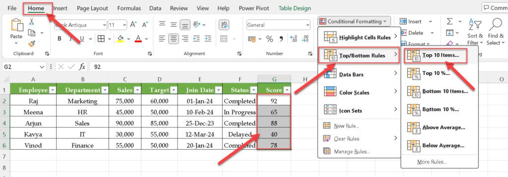
- Change “10” to “3” to highlight the top 3 scores.

- Choose a formatting style and click OK.
The top 3 Sales scores are highlighted.

3. Data Bars
Adds a colored bar inside the cell based on the value. Higher values have longer bars.
- Useful for quick comparison.
Example: Show sales numbers with bar length.
Goal: Show relative performance in Sales visually.
- Select C2:C6 (Sales).
- Go to Conditional Formatting → Data Bars → Gradient Fill → Blue.

Each cell now shows a bar; longer = higher value.
4. Color Scales
Applies gradient colors based on cell values.
- Green → High values
- Red → Low values
Example: Profit/Loss visualization.
Goal: Quickly see high/low scores with colors.
Select G2:G6 (Scores).
Go to Conditional Formatting → Color Scales → Red- Yellow-Green.

High scores are Green, average scores Yellow, low scores Red.
5. Icon Sets
Shows symbols inside cells based on values.
- Arrows (up/down)
- Traffic lights (red/yellow/green)
- Ratings (stars, bars, flags)
Example: Show arrows for growth percentage.
Goal: Show project status visually.
- Select C2:C6 (Sales).
- Go to Conditional Formatting → Icon Sets → Traffic Lights.
High = Green, Medium = Yellow, Low = Red.
6. New Rule (Custom Rule)
- You can create your own conditions with formulas.
Example:
Goal: Identify employees whose Sales are less than Target.
- Select both Sales and Target columns → C2:D6.

- Go to Home → Conditional Formatting → New Rule → Use a Formula.
- Under edit the rule description Enter formula =C2<D2

- Click on format option and Choose a red fill color.
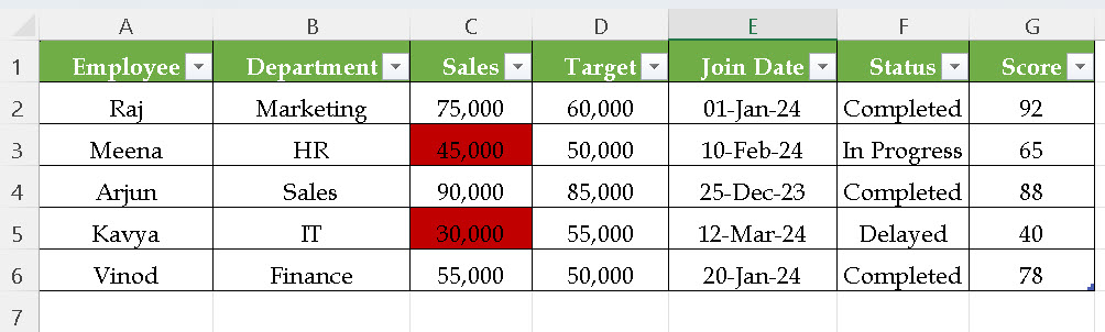
Now all Sales less than Target are highlighted in red.
How to Remove Conditional Formatting?
- Go to Home Tab → Conditional Formatting → Clear Rules.
- Choose:
- Clear rules from selected cells.
- Clear rules from the entire sheet.
Tips for Using Conditional Formatting
- Don’t overuse it. Too many colors can make your sheet messy.
- Use simple rules for quick insights and formulas for advanced needs.
- Great for dashboards, reports, and trend analysis.
Conditional Formatting makes your Excel sheets smarter and more interactive. Whether you want to highlight important numbers, visualize data trends, or spot errors, this tool can save time and improve your data analysis. Start with simple rules like highlighting values and then move on to custom formulas for advanced use.