How to Add Superscripts and Subscripts to Text in Excel:

Have you ever tried typing a chemical formula like H₂O, CO₂, or x² in Excel?

You type the text, but the numbers stay on the same line instead of appearing above or below the letters.

The result doesn’t look right.

This is a common problem, especially if you’re creating scientific reports, mathematical worksheets, engineering documents or any file that requires special formatting.

The good news is that Excel lets you format selected characters as Superscript or Subscript in just a few clicks.

Although Excel doesn’t display dedicated Superscript and Subscript buttons on the Ribbon by default, there are several easy ways to apply these formatting options.

In this guide, you’ll learn what superscripts and subscripts are, when to use them, and the easiest methods to add them in Microsoft Excel.

What Are Superscripts and Subscripts?

Before learning the steps, let’s quickly understand the difference between these two formatting options.

A Superscript is a character that appears slightly above the normal text.

For example:

• x²
• 10³
• cm²

Superscripts are commonly used for:

• Mathematical powers
• Square and cubic units
• Footnotes
• Scientific equations

A Subscript is a character that appears slightly below the normal text.

For example:

• H₂O
• CO₂
• H₂SO₄

Subscripts are mainly used for:

• Chemical formulas
• Scientific notation
• Mathematical expressions
• Physics equations

These formatting options only change the appearance of the text. They don’t change the value stored in the cell.

When Should You Use Superscript or Subscript in Excel?

Although Excel is mainly used for calculations, many people also use it to prepare reports, project documentation, invoices, laboratory records and educational worksheets.

In these situations, properly formatted text makes your worksheet look much more professional.

You may need Superscript or Subscript when you’re working with:

• Chemical formulas like H₂O or CO₂
• Mathematical expressions such as x² or y³
• Engineering calculations
• Scientific research reports
• Footnotes and references
• Square or cubic units like m² and m³

Instead of leaving the numbers on the same line, formatting them correctly makes the information easier to read.

Method 1: Use the Format Cells Dialog Box:

The Format Cells dialog box is the easiest and most commonly used method for adding superscripts or subscripts in Excel.

If you only need to format a few characters, this method is usually the best choice.

Step 1: Enter Your Text:

Type the text into a cell.

For example: H2O or x2

Step 2: Edit the Cell:

Double-click the cell or press F2 to edit it.

Now select only the character that you want to format.

For example:

• Select only the 2 in H2O
• Select only the 2 in x2

Don’t select the entire text.

Only the selected characters will be formatted.

Step 3: Open the Format Cells Window:

There are two easy ways to open the Format Cells dialog box.

Option 1:

Right-click the selected text and choose the Format Cells option from the context menu.

Option 2:

Press the keyboard shortcut: Ctrl + 1

This shortcut works almost everywhere in Excel and is much faster.

Step 4: Apply Superscript or Subscript:

Inside the Format Cells window:

• Open the Font tab.
• Under Effects, you’ll see two options:
• Superscript
• Subscript

Choose the option you need.

Click OK.

If you selected Subscript, your text changes like this:

H₂O

If you selected Superscript, your text becomes:

x²

That’s all there is to it.

This method works perfectly whenever you only need to format a small amount of text.

Method 2: Add Superscript and Subscript to the Ribbon:

If you use Superscript or Subscript regularly, opening the Format Cells dialog box every time can become repetitive.

A better option is to add these commands directly to the Ribbon.

Once you’ve done that, formatting text becomes much faster because the commands are always available.

Customize the Ribbon:

Step 1: Open Ribbon Customization:

Right-click anywhere on the Ribbon.

Choose:

Customize the Ribbon

The Excel Options window opens.   

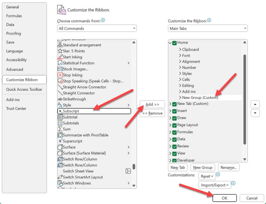
In the Excel Options window, on the right side, you’ll see a list of commands and a representation of the Ribbon.

Step 2: Create a New Group:

In the right pane, Choose the tab where you want to place the commands.

Most people add them to the Home tab.

Click the “New Group” button to create a new group within the selected tab.

You can rename this group if you’d like.

For example:

• Text Formatting
• Special Formatting
• Font Tools

This makes it easier to find later.

Step 3: Add the Commands:

In the left pane (the list of commands), change the dropdown menu to “All Commands.”

Scroll down until you find:

• Superscript
• Subscript

Select each one and click Add.

They’ll now appear inside your new Ribbon group.

Step 4: Save Your Changes:

Click OK.

You’ll now see your new buttons on the Ribbon.

Whenever you need Superscript or Subscript, simply:

• Select the character
• Click the appropriate button

No need to open the Format Cells dialog box again.

Rename and Rearrange:

• To make your custom group more meaningful, you can right-click on it and choose “Rename” to give it a suitable name.

• You can also use the up and down arrows to rearrange the commands within the custom group.

• Click “OK” to save your customizations.

Method 3: Add Superscript and Subscript to the Quick Access Toolbar:

If you frequently use Superscript or Subscript, adding them to the Quick Access Toolbar (QAT) can save you even more time.

The Quick Access Toolbar is always visible, regardless of which Ribbon tab you’re using. This means you can apply formatting with just one click.

Step 1: Open Quick Access Toolbar Settings:

Click the small Customize Quick Access Toolbar arrow at the top-left corner of Excel.

From the menu, select:

More Commands

The Excel Options window will open.

Step 2: Choose the Commands:

From the Choose commands from drop-down list, select:

All Commands

Now scroll through the list until you find:

• Superscript
• Subscript

Select each command and click Add.

The commands will appear on the right side, which represents your Quick Access Toolbar.

Step 3: Save the Changes:

Click OK.

You’ll now see both Superscript and Subscript icons in the Quick Access Toolbar.

Whenever you need them:

• Edit the cell.
• Select the character.
• Click the required button.

This is one of the fastest ways to apply text formatting if you use these options regularly.

Method 4: Insert Special Symbols in Excel:

Sometimes you don’t need to format existing text.

Instead, you may simply want to insert special characters such as:

• ²
• ³
• °
• µ
• α
• β

In these situations, you can use Excel’s Symbol feature.

Step 1: Select the Cell:

Click the cell where you want to insert the symbol.

Step 2: Open the Symbol Window

Go to the Insert tab.

In the Symbols group, click Symbol.

A dialog box will appear with hundreds of special characters.

Step 3: Choose the Symbol:

Browse through the available symbols or select a different font if needed.

Choose the symbol you want.

Click Insert.

Then close the dialog box.

The selected symbol will appear in your worksheet.

This method is useful when you need to insert specific symbols or mathematical notations as superscripts or subscripts.

Which Method Should You Use?

Excel offers several ways to add Superscript and Subscript, but the best method depends on how often you use them.

If You…	Best Method
Need Superscript or Subscript occasionally	Format Cells dialog box
Use them frequently	Add them to the Ribbon
Want the fastest access	Add them to the Quick Access Toolbar
Need special characters like ² or °	Insert Symbol

For most users, the Format Cells method is the simplest and easiest option.

If you’re regularly creating scientific or mathematical documents, customizing the Ribbon or Quick Access Toolbar can save a lot of time.

Things to Remember:

Before using Superscript or Subscript in Excel, keep these points in mind.

• You can format only part of the text inside a cell. For example, in H₂O, you can format only the number 2 as a subscript.
• Superscript and Subscript only change how the text looks. They don’t change the actual value stored in the cell.
• These formatting options do not affect calculations or formulas. They are used only for display purposes.
• You can’t apply Superscript or Subscript to part of a formula. Excel formulas return values, not specially formatted characters.
• If you edit the formatted text later, you may need to apply the Superscript or Subscript formatting again.

Keeping these points in mind will help you avoid confusion while working with formatted text.

Common Mistakes Beginners Make:

Many Excel beginners run into small issues when using Superscript or Subscript for the first time.

Here are some of the most common ones.

Selecting the Entire Cell:

• Many users select the whole cell instead of only the character they want to format.
• As a result, the entire text becomes Superscript or Subscript.
• Always edit the cell first, then highlight only the required character.

Trying to Format Formula Results:

• Superscript and Subscript only work with text.
• They can’t be applied to part of the result returned by a formula.
• If you need special formatting in calculated results, you’ll need a different approach.

Looking for Ribbon Buttons:

• Many beginners spend time searching the Home tab for Superscript and Subscript buttons.
• By default, Excel doesn’t include these commands on the Ribbon.
• You can either use the Format Cells dialog box or add the commands yourself using Ribbon customization.

Frequently Asked Questions (FAQs):

Can I apply Superscript to only one character in a cell in Excel?

Yes.

Edit the cell, select only the character you want to format, open the Format Cells dialog box, and choose Superscript.

Can I apply Subscript to part of the text?

Yes. You can format individual letters, numbers, or symbols without affecting the rest of the text.

Is there a keyboard shortcut for Superscript in Excel?

There isn’t a direct keyboard shortcut.

However, you can quickly open the Format Cells dialog box by pressing Ctrl + 1, then choose Superscript or Subscript from the Font tab.

Can I use Superscript or Subscript in Excel formulas?

No. These formatting options only affect text. They can’t be used inside formulas or calculations.

Can I add Superscript and Subscript buttons to the Ribbon?

Yes. Excel allows you to customize the Ribbon and the Quick Access Toolbar by adding these commands for faster access.

Superscript and Subscript are small formatting features, but they can make a big difference in how your worksheets look.

Whether you’re creating chemical formulas like H₂O, mathematical expressions like x², or scientific reports, using the correct formatting makes your data easier to read and more professional.

Now that you know the different ways to add Superscript and Subscript in Excel, you can format your worksheets with confidence and create documents that are both accurate and professional.