7 Quick Methods to Add Serial Numbers in Excel:

Serial numbers play a significant role in Excel data. If you’re working with a large set of data, it is always recommended to give a serial number to each row of your data.  They provide a unique identity to each entry in the table.

Adding serial numbers manually to each row is a big task but Excel makes it easy. You can add serial numbers for each entry of your data or in the table easily.

In this post, I’ll share quick methods to add serial numbers to your data in Excel.

Use Fill Handle to Generate the Serial Numbers:

Simply follow the below steps to add the serial numbers.

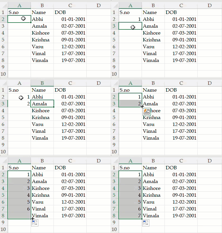
1. Enter 1 in the first cell.
2. Enter 2 in the second cell.
3. Select both cells and move the cursor to the lower–right corner.
4. Now the pointer turns into a plus sign.
5. Drag the fill handle down to the cell where you want the last serial number.
6. After getting as many serial numbers as you want, just release the mouse.

Inserting 1 & 2 in the cells is a must to generate the serial numbers using the Fill Handle.

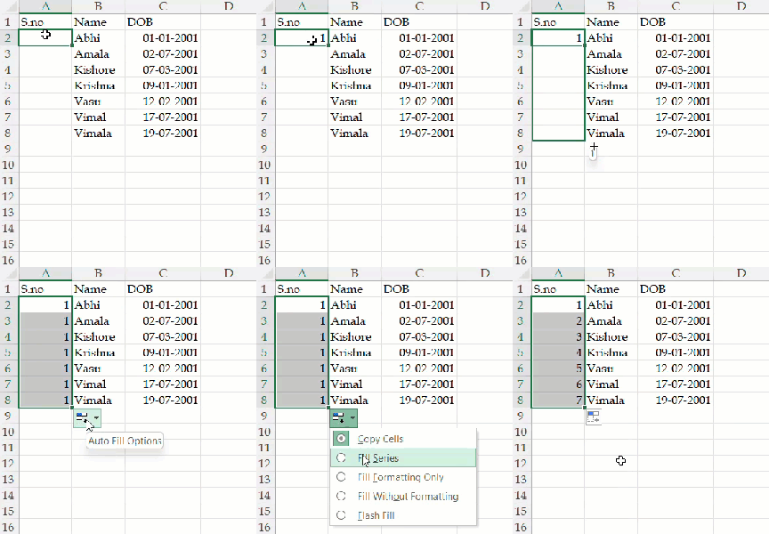
If you enter 1 in the cell and drag the cursor down. It will repeat 1 in every cell.

In this situation, just click on the auto-fill option to open the menu and click on the Fill series option to generate the serial numbers.

Note: This is not the dynamic way to generate the serial numbers. You need to repeat the fill handle process to change the serial numbers each time when you add new rows at the bottom and insert or delete the rows in between.

Pro tip: If you’re working with a large set of data, dragging the fill handle till the end of the data is boring and time taking. In that situation, you can double-click on the fill handle to fill the series till the end.

Use the Fill Series Command:

The fill series command will come in handy if you want to add serial numbers to a particular number.

Let’s say, you want to generate serial numbers up to 100 or 1000, you can use the Fill series command to do it in one go.

Let’s check, how?

1. Go to a cell where you want to start the number and add 1.
2. Select that cell, Go to the Home tab on the ribbon and click on the Fill drop-down button under the Editing group.

3. Click on the Series command to open the Series dialog box.
4. Under the Series in option, select columns.
5. Add a Stop value of 100 or 1000 whatever you want.

6. Click OK.

Using this method, you can generate serial numbers up to 1048576 if you start 1 from the A1 cell.

Note: This is also not the dynamic way to generate the serial numbers. You need to repeat the process to change the serial numbers if you want to extend the list and insert or delete the rows in between.

Add One to The Previous Number:

Excel is all about calculations. Using the calculations, we are going to generate the serial numbers for your data in Excel.

1. Go to a cell where you want to start the number and add 1. Here I’m adding 1 to cell A2.
2. Then in the next row, add the below formula.

                =A2+1

3. Now select the second cell and double-click on the fill handle to fill the series till the end.

Note: This is also not the dynamic way to generate the serial numbers. If you delete any row, you’ll get #REF error for all the below rows. At that time, you need to copy the above formula to balance cells to change the serial numbers.

Use ROW Function:

Using the ROW function, we can easily create perfect serial numbers in Excel.

1. Go to a cell and add the below formula where C1 refers to the column heading.

                   =ROW()-ROW($C$1)

2. Now select the same cell and double-click on the fill handle to fill the series till the end.

If you add only the =ROW() formula in the cell, the row function returns to the row number of the current row. So, if you add this formula in the 8^th row, it will start generating the serial numbers from 8. In order to generate the serial numbers from 1, we need to subtract the before row. Here I’m subtracting S.NO heading cell using the above formula to generate the serial numbers from 1.

Note: This is a dynamic way to generate serial numbers. Serial numbers will automatically get updated if you insert or delete the rows in between.

Use COUNTA Function:

This is another formula option that will actually count your data entries and generate the serial numbers.

In order to use the COUNTA function, first we need to take a cell that will never contain any blank value. COUNTA function will not count the cell that contains blank values.

1. Go to the cell where you want to start the serial number. Here I need the serial number from A3.
2. Add the below formula in the A3 cell where A2 refers to the column heading – a non-blank cell that we never delete that needs here to work the formula.

                  =COUNTA($A$2:A2)

3. Now select the same cell and double-click on the fill handle to fill the series till the end.

Note: This is a dynamic way to generate serial numbers. Serial numbers will automatically get updated if you insert or delete the rows in between.

Use SEQUENCE Function:

Previously we have used the COUNTA function. If we use the COUNTA function within the sequence function, we can get the output once without adding code to balance cells.

While using the Sequence function, we need to add a range of cells that contains the values in the formula.

1. Go to the cell where you want to start the number.
2. Add the below formula in that cell. Here I need serial numbers from A2 to A10. So I’ve added the range B2:B10 in the formula.

            =SEQUENCE(COUNTA(B2:B10))

That’s it. No need to add the formula to balance cells.

Note: This is also a dynamic way to generate the serial numbers. Serial numbers will automatically get updated if you insert or delete the rows in between.

Use SUBTOTAL Function:

The SUBTOTAL function returns the values based on the cells that are visible and ignores the cells that are not visible in the filter results. This means the serial numbers get updated when you filter the data.

1. Go to a cell where you want the first serial number. Here I need the serial number from A2.
2. Add the below formula in A2.

             =SUBTOTAL(3,$B$2:B2)

3. Now select the same cell and double-click on the fill handle to fill the series till the end.

This formula also works like the COUNTA function but the only difference is unlike in the COUNTA function the serial numbers will get updated based on the cells that are visible when you filter the data.

Note: This is the best and most dynamic way to generate the serial numbers. Serial numbers will automatically get updated, if you insert or delete the rows in between and also when filter the data.